The length of genomes varies widely. For example, a simian virus (SV40) DNA genome is 5,200 base pairs (bp), a human mitochondrial genome is 16,569 bp, the smallest human chromosome, chr21, is 46,709,984 bp, and the largest, chromosome 1, is 248,956,422 bp

Sanger and Maxam and Gilbert’s methods can produce sequence lengths from 500 to 1,000 bases. Highly parallel high throughput platforms produce sequence fragments ranging from 20 bp to 500 bp. Long-read sequencing, such as PacBio and Oxford Nanopore can produce read lengths up to a few tens of kilobases.

Organism	Approximate genome length
Bacteriophages and viruses	2kb - 1Mb
Prokaryotic genomes	500 kb - 12Mb
Eukaryotic genomes	10 Mb - >100 000 Mb

So, by using long-read sequencing it is theoretically possible to sequence short viral, bacteriophage, and some prokaryotic genomes without a need for sequence assembly but fall way short of the lengths of large chromosomes and genomes. However, it is still desirable to add short-read sequencing to increase the accuracy as we see in the subsequent sections.

Therefore, the method of choice is to generate many overlapping sequence fragments that can be assembled together by pairing identical sequence stretches. We do this by first making many copies of a genome and then randomly breaking all the copies into short overlapping fragments.

Since many of the fragments are overlapping, it is possible to assemble all the fragments back together by observing which portions of the fragments are identical. The identical, overlapping parts of the sequence fragments should represent the same location of a genome (Figure 1). This is the core idea but the approach also presents many complications. You will understand the reason after finishing this tutorial.

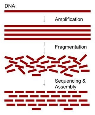
Figure 1. Simplified concept of DNA sequencing.

Animation 1. Animation of copying and breaking DNA for genome assembly.

Sequencing Coverage

The sequencing coverage describes the number of times the target genome is sequenced. The original DNA is amplified, i.e., copied several times and randomly broken into many overlapping fragments (Figure 1). These fragments are then sequenced. The number of reads (sequenced fragments) multiplied by the average length of the reads gives us the total DNA length sequenced.

Mean Raw Read Depth

For example, the length of a haploid human genome is about three billion base pairs (3Gb) and if we sequence and we want to achieve 50 times coverage (50X), we need to sequence enough fragments to get in total 50 x 3Gb of sequence.

So, if the average read length is 200 bp we need to sequence 50 x 3Gb / 200bp = 750,000,000 fragments. Thus, we can calculate the sequence coverage or redundancy as follows

C = N x L / G

Where C is the coverage, N is the average read length, and G is the length of the genome we want to sequence. If we insert the values of the above example, G = 3Gb, L = 200 bp, and N = 750,000,000, the Equation 1 gives us the coverage, C = 200bp x 750,000,000 / 3 Gb = 50, as expected.

Note that C is the average coverage and works as expected only if the genome is broken into fragments as randomly as possible. Furthermore, we only sequence as many fragments that are required to achieve the desired coverage, not all of them. Therefore, the selection of which fragments we sequence must also be random.

The higher the average coverage is the lower the probability that some genomic regions lack coverage. A random sequencing results in a sequence coverage that follows the Poisson distribution; Thus, the coverage varies from one genomic region to another, also termed as the mapped read depth (Figure 2).

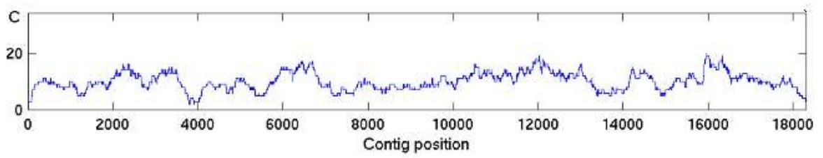
Figure 2. An example of an average 10X coverage along a contiguous sequence (contig).

Mean Mapped Read Depth

An ideal assembled coverage distribution, i.e., the variation in the mapped read depth should resemble the Poisson distribution as in Figure 3. For several reasons the mapped read depth can deviate from the ideal (Figure 4). One common cause is repeated regions in genomes.

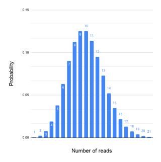
Figure 3. Read coverage according to Poisson with an average of 10.

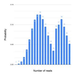
Figure 4. An example of non-Poisson read coverage. The mapped read depth can deviate from the ideal Poisson distribution for many different reasons.

Non-random selection of reads results in biased sequence coverage where some genomic regions may have extremely high coverage and some may lack coverage altogether. So, the randomness is important also because sequence assembly programs tend to incorrectly assemble highly similar or identical repeats into a single alignment, also resulting in high coverage.

Bias in sequence coverage

In practice, the sequencing coverage will deviate from the ideal uniform distribution over the whole genome. Unfortunately, all sequencing technologies produce biases in varying degrees and types. Despite a high sequence coverage, some regions may not be covered at all resulting in unwanted gaps.

On the other hand, biased sequence coverage may mislead us to incorrectly conclude that a high coverage region is caused by erroneously assembled repeated regions or at least will make it difficult to assess the underlying cause. See below “What complicates genome assembly? Repeated regions.”

Examples of sequence coverage biases

Methods that use bacterial cloning are subject to the loss sequences that are toxic to the bacterial host. Besides, all methods that use PCR amplification are subject to loss of sequence coverage of extreme GC-rich regions. In addition to GC-extremes, Sanger sequencing produces errors that are specific to palindromic regions and inverted repeats. Sequencing methods that do not use amplification, such as Pacific Biosciences, are not affected by amplification biases.

Illumina sequencing and other similar technologies may lose coverage in both high and low GC content sequences stretch. Besides, Illumina produces some errors that are DNA strand-specific. Long homopolymer stretches are an obstacle for terminator free chemistries, such as Ion Torrent and 454 methods. Specifically, they have difficulties in producing an accurate count of bases within homopolymer regions.

All biases, lack of coverage, and erroneous sequences hamper assembly programs to correctly compute a correct sequence assembly.

How to select proper coverage depends on the sequencing method, the purpose, and of course, the amount of money one can spend. However, further details on sequencing coverage is a topic for another tutorial.

It is important to evaluate the quality of genome assemblies. Learn more about it in the Tutorial: Genome assembly Quality Metrics.

Paired-end sequencing and mate-pairs

To overcome the limitations of limited read lengths, we can sequence fragments from both ends. By selecting fragments of a specific size, longer than the read length, and sequencing both ends, we will know how far apart the two sequenced ends are (Figure 3). The knowledge of the distance between a pair of reads helps assembly programs to assemble repeated regions.

Paired-end sequencing is commonly used in de novo genome sequencing, to finish complex sequence rearrangements, repeated regions, and identification of structural variants.

Two basic methods exist for paired-end sequencing. 1. Short insert paired-end sequencing, yielding lengths from 200bp to 800bp. 2. Long insert paired-end sequencing, usually 2kb to 5kb long but can be even longer. These long insert paired-ends are also called mate-pairs (Figure 5).

One may wonder why not produce all fragments as mate-pairs alternatively use long-read sequencing that can produce several kilobases of contiguous sequence? The reason is the cost. High-throughput short-read sequencing is still much cheaper than the alternatives and is used to provide overall coverage. Therefore, the majority of the sequence coverage is based on short-reads and only a relatively small portion of additional coverage by short- and long-insert paired-end sequencing.

A combination of short-insert paired-end and mate-pairs provide coverage to span across repeated regions and to resolve structural variants. An alternative is of course to use long-read sequencing but it is a matter of available funding since long-read sequencing is still relatively expensive in comparison.

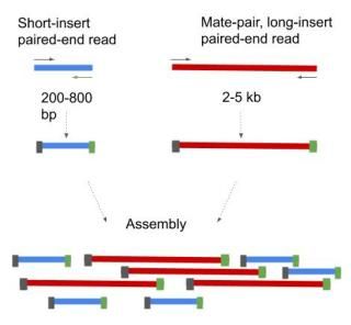
Figure 5. Short- and long-insert paired-ends. The long-insert paired-ends are also termed as mate-pairs.

What complicates genome assembly?

Repeated regions

Repeats and duplicated regions are the main devils making the assembly task difficult. In general, assembly algorithms are able to handle repeats that are shorter than the average read length. Although, not all the time 100% correct. Depending on the specific algorithm and parameter settings a small portion of fragments containing short repeat may still end up in the wrong location. This can happen when only a few bases in a flanking region do not match the consensus sequence while the rest of the fragment matches more or less perfectly.

When the bases of a fragment do not match the rest of the alignment, we must consider a few different causes for this. 1. The differences are caused by sequencing errors, 2. The fragment is a repeat belonging to a different genomic location (Figure 5), or 3. The fragment is in a correct location but contains polymorphism among the homologous chromosomes (Figure 6).

If the base qualities are low, i.e., the probability of errors is above a set threshold, the software will label these as errors (1). However, in the case of the bases having a low error probability, then the fragment is likely to originate from a different genomic location (2) (Figure 5), or the differences are caused by polymorphism (3) (Figure 6).

In the cases where the differences are caused by short flanking regions of erroneously assembled fragments, the number of such reads is in general low. In addition, the differences appear at the beginning or at the end of the sequenced fragments. In comparison, if the differences are due to polymorphism among homologs, we should see a higher number of fragments containing the same sequence. We can use these facts to determine the correct case.

Note though that this is theoretical and the reality is usually more complicated. Particularly when we encounter a mix of all three cases in the same location.

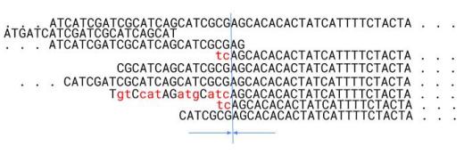
Figure 5. Example of differences likely due to erroneous alignment of repeated regions. The blue line marks the repeat boundary. The left side of the boundary consists of non-repeated sequences.

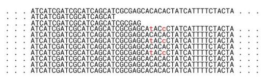
Figure 6. Example of differences in alignment caused by polymorphism.

Repeats that are longer than the length of the sequenced fragments are more problematic because only the flanking regions are unique and the reads are not long enough to cover entire repeats.

The repeated regions can be identical or nearly identical in varying degrees and they can be interspersed in the genome or appear in tandem, repeated one or more times. For example, the human genome contains 45% transposons, 5% percent of large duplications, and about 3% micro- and minisatellites that are shorter than 100 base pairs. Thus, about half of the human genome is made up of repetitive sequences.

Animation 2. How repeated sequence regions complicate sequence assembly.

Base-calling errors or sequencing errors

None of the DNA sequencing methods are free of errors and the error rate varies depending on the sequencing method. The errors may consist of erroneous base calls, missed bases, and even erroneous addition of bases. In other words, all possible errors with different biases depending on the platform. In particular single-molecule sequencing error rate is high, about 5% to 15%, compared to short-read and Sanger sequencing methods.

Since accurate sequencing is an essential prerequisite to not only achieve correct assemblies but further analyses, such as detection of single-nucleotide polymorphism (SNP), and the assessment of structural variation. Therefore, several teams have developed error correction software that attempt to rectify sequencing errors prior to the assembly step. However, they are not able to correct all the errors. For example, many such algorithms rely on the sequencing errors being randomly distributed and thus fail specific biases that produce similar errors that are not random.

Also, the estimation of base quality values or the probability of a base being erroneously called, are valuable in tackling sequencing errors. All major sequencing platforms provide base-wise quality values. But, as is the case most of the time, nothing is 100% perfect. First, the estimates are not perfectly correct, and second, they consist of probabilities.

How assemblers handle quality values, depends on the specific parameter settings and the algorithm. After all, in each specific alignment case, the question is how do you handle a base that has an error probability of, for example, 10%, 5%, or 0.1%. In each case, the base may be correct or incorrect.

Phred quality scores are commonly used and defined as

Q = -10 Log₁₀ P,

Where Q is the quality and P is the error probability. The quality scores range from 4 to 60. For example, score 10 means that the error probability is 1 in 10, the score 20 means 1 error in 100, and the score 60 the error probability 1 in 1,000,000.

We have a chance to correctly assemble identical repeats only if we have contiguous sequences that span over the entire repeated stretches including the flanking no-repeated parts. If we lack contiguous sequences spanning over the entire repeated regions, sequencing errors can confuse assemblers to resolve parts of de facto identical repeats into several separate contigs.

Repeated regions vary in degree of similarity. Nearly identical repeats are also cumbersome to assemble correctly. Due to only a few differences between repeat copies and the presence of sequencing errors, it is often difficult to make a distinction between a real difference and a sequencing error.

Unknown orientation

DNA is double-stranded and in the fragmentation process, we lose the information of which DNA strand each fragment originates. Given a good sequence coverage, it is possible to solve the orientation problem. The only drawback is that we have to convert all the sequences also into reverse complementary sequences, thereby doubling the number of sequences; Thus, adding computing time.

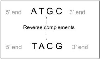
Figure 7. Reverse complementary sequences.

See also in-house software to make reverse complementary sequences at RevComp.

Incomplete coverage

As described in the section Examples of sequence coverage biases (link), some genomic locations may have lower than expected coverage or lack coverage altogether. Theoretically, increasing the average coverage, i.e., sequencing more fragments, will decrease the chance that any region lacks coverage. Due to biases in the sampling process itself and platform-specific biases, the actual coverage will deviate from the theoretically calculated coverage.

Contamination

In cases where we use bacterial cloning, for example, E. coli, the most likely source of contamination is the host sequences mixed with genomic sequences. However, mistakes happen and it is a good practice to always filter the sequences even when cloning is not used.

See also the list of whole genome assembly (WGA) tools in our database section.

Genome assembly Quality Metrics

Sequence Assembly Practical

Pair-wise sequence alignment

Pair-wise sequence alignment methods

Please, send comments and suggestions. Suggest for example a topic you would like to see or any improvements in the content. We will not spam you with emails!

References

Haubold B, Wiehe T. “How repetitive are genomes?” BMC Bioinformatics. 2006;7:541. Published 2006 Dec 22. DOI:10.1186/1471-2105-7-541

Wetzel J, Kingsford C, Pop M. “Assessing the benefits of using mate-pairs to resolve repeats in de novo short-read prokaryotic assemblies.” BMC Bioinformatics. 2011;12:95. Published 2011 Apr 13. DOI:10.1186/1471-2105-12-95

Wang Z, Fang B, Chen J, et al. “De novo assembly and characterization of root transcriptome using Illumina paired-end sequencing and development of cSSR markers in sweet potato (Ipomoea batatas).” BMC Genomics. 2010;11:726. Published 2010 Dec 24. DOI:10.1186/1471-2164-11-726

Fu N, Wang Q, Shen HL. “De novo assembly, gene annotation, and marker development using Illumina paired-end transcriptome sequences in celery (Apium graveolens L.).” PLoS One. 2013;8(2):e57686. DOI:10.1371/journal.pone.0057686

Ramos RT, Carneiro AR, de Castro Soares S, et al. “High efficiency application of a mate-paired library from next-generation sequencing to postlight sequencing: Corynebacterium pseudotuberculosis as a case study for microbial de novo genome assembly.” J Microbiol Methods. 2013;95(3):441-447. DOI:10.1016/j.mimet.2013.06.006

Chin CS, Alexander DH, Marks P, et al. “Nonhybrid, finished microbial genome assemblies from long-read SMRT sequencing data.” Nat Methods. 2013;10(6):563-569. DOI:10.1038/nmeth.2474

Wang XV, Blades N, Ding J, Sultana R, Parmigiani G. “Estimation of sequencing error rates in short reads. BMC Bioinformatics.” 2012;13:185. Published 2012 Jul 30. DOI:10.1186/1471-2105-13-185

Albaradei S, Magana-Mora A, Thafar M, et al. “Splice2Deep: An ensemble of deep convolutional neural networks for improved splice site prediction in genomic DNA.” Gene X. 2020;5:100035. Published 2020 May 13. DOI:10.1016/j.gene.2020.100035

Iadarola B, Xumerle L, Lavezzari D, et al. “Shedding light on dark genes: enhanced targeted resequencing by optimizing the combination of enrichment technology and DNA fragment length.” Sci Rep. 2020;10(1):9424. Published 2020 Jun 10. DOI:10.1038/s41598-020-66331-z

Noakes MT, Brinkerhoff H, Laszlo AH, et al. “Increasing the accuracy of nanopore DNA sequencing using a time-varying cross membrane voltage.” Nat Biotechnol. 2019;37(6):651-656. DOI:10.1038/s41587-019-0096-0

Luo R, Sedlazeck FJ, Lam TW, Schatz MC. “A multi-task convolutional deep neural network for variant calling in single molecule sequencing.” Nat Commun. 2019;10(1):998. Published 2019 Mar 1. DOI:10.1038/s41467-019-09025-z

Francis F, Dumas MD, Davis SB, Wisser RJ. “Clustering of circular consensus sequences: accurate error correction and assembly of single molecule real-time reads from multiplexed amplicon libraries.” BMC Bioinformatics. 2018;19(1):302. Published 2018 Aug 20. DOI:10.1186/s12859-018-2293-0

Ta M, Yin C, Smith GL, Xu W. “A Workflow to Improve Variant Calling Accuracy in Molecular Barcoded Sequencing Reads.” J Comput Biol. 2019;26(1):96-103. DOI:10.1089/cmb.2018.0110

Ross MG, Russ C, Costello M, et al. “Characterizing and measuring bias in sequence data.” Genome Biol. 2013;14(5):R51. Published 2013 May 29. DOI:10.1186/gb-2013-14-5-r51

Sanger F, Nicklen S, Coulson AR. “DNA sequencing with chain-terminating inhibitors.” Proc Natl Acad Sci U S A. 1977;74(12):5463-5467. DOI:10.1073/pnas.74.12.5463

Collins J. “Instability of palindromic DNA in Escherichia coli.” Cold Spring Harb Symp Quant Biol. 1981;45 Pt 1:409-416. DOI:10.1101/sqb.1981.045.01.055

Wyman AR, Wertman KF. “Host strains that alleviate underrepresentation of specific sequences: overview.” Methods Enzymol. 1987;152:173-180. DOI:10.1016/0076-6879(87)52017-1

Leach D, Lindsey J. “In vivo loss of supercoiled DNA carrying a palindromic sequence.” Mol Gen Genet. 1986;204(2):322-327. DOI:10.1007/BF00425517

Chissoe SL, Marra MA, Hillier L, Brinkman R, Wilson RK, Waterston RH. “Representation of cloned genomic sequences in two sequencing vectors: correlation of DNA sequence and subclone distribution.” Nucleic Acids Res. 1997;25(15):2960-2966. DOI:10.1093/nar/25.15.2960

Keith JM, Cochran DA, Lala GH, Adams P, Bryant D, Mitchelson KR. “Unlocking hidden genomic sequence.” Nucleic Acids Res. 2004;32(3):e35. Published 2004 Feb 18. DOI:10.1093/nar/gnh022

Sorek R, Zhu Y, Creevey CJ, Francino MP, Bork P, Rubin EM. “Genome-wide experimental determination of barriers to horizontal gene transfer.” Science. 2007;318(5855):1449-1452. DOI:10.1126/science.1147112

Godiska R, Mead D, Dhodda V, et al. “Linear plasmid vector for cloning of repetitive or unstable sequences in Escherichia coli.” Nucleic Acids Res. 2010;38(6):e88. DOI:10.1093/nar/gkp1181

Kimelman A, Levy A, Sberro H, et al. “A vast collection of microbial genes that are toxic to bacteria.” Genome Res. 2012;22(4):802-809. DOI:10.1101/gr.133850.111

Bentley DR, Balasubramanian S, Swerdlow HP, et al. “Accurate whole human genome sequencing using reversible terminator chemistry.” Nature. 2008;456(7218):53-59. DOI:10.1038/nature07517

Dohm JC, Lottaz C, Borodina T, Himmelbauer H. “Substantial biases in ultra-short read data sets from high-throughput DNA sequencing.” Nucleic Acids Res. 2008;36(16):e105. DOI:10.1093/nar/gkn425

Aird D, Ross MG, Chen WS, et al. “Analyzing and minimizing PCR amplification bias in Illumina sequencing libraries.” Genome Biol. 2011;12(2):R18. DOI:10.1186/gb-2011-12-2-r18

Oyola SO, Otto TD, Gu Y, et al. “Optimizing Illumina next-generation sequencing library preparation for extremely AT-biased genomes.” BMC Genomics. 2012;13:1. Published 2012 Jan 3. DOI:10.1186/1471-2164-13-1

Quail MA, Smith M, Coupland P, et al. “A tale of three next generation sequencing platforms: comparison of Ion Torrent, Pacific Biosciences and Illumina MiSeq sequencers.” BMC Genomics. 2012;13:341. Published 2012 Jul 24. DOI:10.1186/1471-2164-13-341

Harismendy O, Ng PC, Strausberg RL, et al. “Evaluation of next generation sequencing platforms for population targeted sequencing studies.” Genome Biol. 2009;10(3):R32. DOI:10.1186/gb-2009-10-3-r32

Stein A, Takasuka TE, Collings CK. “Are nucleosome positions in vivo primarily determined by histone-DNA sequence preferences?” Nucleic Acids Res. 2010;38(3):709-719. DOI:10.1093/nar/gkp1043

Nakamura K, Oshima T, Morimoto T, et al. “Sequence-specific error profile of Illumina sequencers.” Nucleic Acids Res. 2011;39(13):e90. DOI:10.1093/nar/gkr344

Rothberg JM, Hinz W, Rearick TM, et al. “An integrated semiconductor device enabling non-optical genome sequencing.” Nature. 2011;475(7356):348-352. Published 2011 Jul 20. DOI:10.1038/nature10242

Margulies M, Egholm M, Altman WE, et al. “Genome sequencing in microfabricated high-density picolitre reactors” [published correction appears in Nature. 2006 May 4;441(7089):120. Ho, Chun He [corrected to Ho, Chun Heen]]. Nature. 2005;437(7057):376-380. DOI:10.1038/nature03959

Loman NJ, Misra RV, Dallman TJ, et al. “Performance comparison of benchtop high-throughput sequencing platforms” [published correction appears in Nat Biotechnol. 2012 Jun;30(6):562]. Nat Biotechnol. 2012;30(5):434-439. DOI:10.1038/nbt.2198

Huse SM, Huber JA, Morrison HG, Sogin ML, Welch DM. “Accuracy and quality of massively parallel DNA pyrosequencing.” Genome Biol. 2007;8(7):R143. DOI:10.1186/gb-2007-8-7-r143

Merriman B; Ion Torrent R&D Team, Rothberg JM. “Progress in ion torrent semiconductor chip based sequencing” [published correction appears in Electrophoresis. 2013 Feb;34(4):619]. Electrophoresis. 2012;33(23):3397-3417. DOI:10.1002/elps.201200424

Drmanac R, Sparks AB, Callow MJ, et al. “Human genome sequencing using unchained base reads on self-assembling DNA nanoarrays.” Science. 2010;327(5961):78-81. DOI:10.1126/science.1181498

Yang X, Chockalingam SP, Aluru S. “A survey of error-correction methods for next-generation sequencing.” Brief Bioinform. 2013;14(1):56-66. DOI:10.1093/bib/bbs015

Ma X, Shao Y, Tian L, et al. “Analysis of error profiles in deep next-generation sequencing data.” Genome Biol. 2019;20(1):50. Published 2019 Mar 14. DOI:10.1186/s13059-019-1659-6

Introduction To Sequence Assembly - The Fundamentals

Why we need sequence assembly?