The Principles of WGS Sequencing and Automated Fragment Assembly

1 Introduction

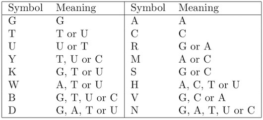
The secret of life is complementarity. Deoxyribonucleic acid, DNA, is a double helix consisting of alternating phosphate and sugar groups. The two chains are held together by hydrogen bonds between pairs of organic bases adenine (A) with thymine (T) and guanine (G) with cytosine (C) (Watson & Crick, 1953). In 1962 James Watson, Francis Crick, and Maurice Wilkins jointly received The Nobel Prize in Physiology or Medicine for their determination of the structure of DNA. In 1959, Seymour Benzer presented the idea that DNA and RNA molecules can be seen as linear words over a 4-letter alphabet (Benzer, 1959). It is the order of these letters (bases) that codes for the important genetic information of an organism.

Contents

1 Introduction

1.1 The Human Genome Project

1.1.1 The First WGS Projects

1.2 The Principle of WGS Sequencing

1.2.1 Strategies for Sequencing

1.2.2 The Hierarchical Sequencing (HS) Strategy
or Clone by Clone Sequencing

1.2.3 The Whole Genome WGS (WGS) Strategy

1.2.4 Combining HS and WGS

1.2.5 WGS Sequencing Methods

1.3 Development of WGS Fragment Assembly Tools

2 Milestones in Genome Sequencing

2.0.1 First Cellular Organisms

2.0.2First Multicellular Organism

3 WGS Fragment Assembly Algorithms

3.1 Types of Problems in SequenceAssembly

3.2 Complications in Fragment Assembly

3.3 Base calling

3.4 The Data Quality

3.5 Error Probabilities

3.6 Genome Coverage

3.6.1 Exercises

3.7 Distance Constraints

3.8 FragmentAssemblyProblemModels

3.8.1 The Shortest Common Superstring Model

3.8.2 The Sequence Reconstruction Model

3.8.3 Graphs

3.9 Algorithms

3.9.1 Contamination

3.9.2 Overlap Detection

3.9.3 Contig Layout Determination

3.9.4 Creation of Multiple Alignments

3.9.5 Computation of the Consensus Sequence

4 WGS Fragment Assembly Programs

4.1 Phrap

4.1.1 The Phrap Method

4.1.2 Greedy Algorithm for Layout Construction

4.1.3 Construction of Contig Sequences

References

DNA can be thought of as the language of life, the four letters in an arrangement of words, each word consisting of three letters, codons, that code for amino acids. The codons or words are arranged in sentences that code for specific proteins. The language of DNA dictates which proteins are made, as well as when and how much. In the early days the determination of the nucleotide sequence was a strenuous task and computer programs were implemented to aid in the sequencing process. These, and in continuation attempts to decipher the language of DNA were the seeds that led to the development of the field of bioinformatics. Today vast amounts of data are available for analysis in various databases around the world. The rapid development of bioinformatics was due to the fast development of computer hardware and the need of large genome projects to store, organize and analyze increasing amounts of data. Genome projects were in turn facilitated by the development of improved bioinformatics tools.

1.1 The Human Genome Project

The development of computational solutions to problems in genomics and sequence handling have been crucial to the decision to undertake and successfully carry out the ambitious effort to sequence the whole human genome, approximately three billion base pairs, and the sequencing of many other genomes. The Human Genome Project (HGP) began formally in October 1990 when the Department of Energy (DOE) and National Institute of Health (NIH) presented a joint five-year plan to the U.S. Congress. The document ⁽¹⁾ says, ”improvements in technology for almost every aspect of genomics research have taken place. As a result, more specific goals can now be set for the project.” This international effort was originally estimated to require 15 years and $3 billion. This plan was revised in 1998, when J. Craig Venter, PE Corporation and The Institute of Genomic Research (TIGR) proposed to launch a joint venture that would sequence the entire human genome in three years (Marshall, 1999). In June of 2000, the publicly sponsored Human Genome Project leaders, the private company Celera Genomics, the U.S. President Bill Clinton, and the Prime Minister of Great Britain Tony Blair announced the completion of a ”working draft” sequence of the human genome. A special issue of Nature, Feb. 15, 2001 contains the initial analyses of the draft sequence of the International Human Genome Sequencing Consortium, while a special issue of Science, Feb. 16, 2001, reported the draft sequence reported by the private company, Celera Genomics. The draft sequence is to be improved to achieve a complete, high-quality DNA reference sequence by 2003, two years earlier than originally projected.

1.1.1 The First WGS Projects

In 1965, Robert William Holley and co-workers published the complete sequence of the alanine tRNA from yeast (Holley et al., 1965), a task that took seven years to complete. Since the sequence of only small fragments could be determined, a fragmentation stratagem had to be used. An enzyme obtained from snake venom was used to remove nucleotides one by one from a fragment, to produce a mixture of smaller fragments of all possible intermediate lengths. This mixture was subsequently separated by passing it through a chromatography column. By the determining the identity of the terminal nucleotide of each fraction and the knowledge of its length, it was possible to establish the sequence of the smaller fragments, as well as the sequence of the original large fragment using basic overlapping logic.

The first three WGS sequencing projects were the 6,569 base pair human mitochondrial DNA (Anderson et al., 1981), the bacteriophage λ nucleotide sequence of 48,502 base pairs (Sanger et al., 1982) and the Epstein-Barr virus at 172,282 base pairs (Baer et al., 1984). In the WGS sequencing method (Anderson, 1981; Messing et al., 1981; Deininger, 1983) the sequence is broken into small pieces, since the length of the longest contiguous DNA stretch that can be determined is limited by the length that can be read using an electrophoresis gel. In the bacteriophage λ project, the whole λ genome was sonicated to yield small fragments, (Fuhrman et al., 1981) in order to create a random library of fragmented DNA. These fragments were cloned using a single stranded bacteriophage M13 (Gronenborn & Messing, 1978; Messing et al., 1981) as a vector. This cloning procedure replaced the previous methods. All the sequences were assembled using Rodger Stadens assembly program (Staden, 1982a; Staden, 1982b).

After the introduction of gel electrophoresis based sequencing methods in 1977 by Maxam & Gilbert using chemical degradation of DNA (Maxam & Gilbert, 1977) and chain termination techniques by Frederick Sanger and his colleagues (Sanger et al., 1977), it became possible to determine longer sequences. These techniques allow a routine determination of approximately 300 consecutive bases of a DNA strand in one reaction.

Until the advent of fluorescent sequencing, polyacrylamide slab gel electrophoresis was used together with radioactive 32P, 33P or 35S labels and autoradiographs. Fluorescent labelling, i.e. dyes that can be detected after excitation using a laser, allowed automatic detection of the base sequence (Smith et al., 1986). Regardless of refinements of the sequencing methods, the average fragment length has not grown significantly. In some conditions and using special care it is possible to produce reads that are over 1000 bases long, but only average lengths of about 400 to 800 base pairs are feasible in routine production.

Attempts to increase the sequencing speed and throughput, as well as attempts to lower the cost has led to the development of alternative strategies, such as sequencing by hybridization (Drmanac et al., 1989), Massively Parallel Signature Sequencing (MPSS) (Brenner et al., 2000a; Brenner et al., 2000b), Matrix-assisted Laser Desorption Ionization Time-of-Flight (MALDI-TOF-MS) (Karas & Hillenkamp, 1988), Pyrosequencing (Ronaghi & Nyren, 1998) and the use of Scanning Tunneling Microscopy (Allison et al., 1990). However, none of these methods have as yet contributed to large-scale genomic sequencing due to their short read lengths, but many of them are well suited for e.g. Single Nucleotide Polymorphism (SNP) genotyping. Thus, Sanger sequencing remains the method of choice for large-scale sequencing.

1.2 The Principle of WGS Sequencing

Although the computational problems involved in fragment assembly have been studied almost 30 years, they still continue to receive attention, mainly because of large sequencing projects, such as human genome project and many other projects, necessitates access to efficient algorithms for precise assembly of long DNA sequences and attempts to sequence whole genomes, using the whole genome WGS sequencing approach revealed some limitations in currently used methods. Several genomes have been published as drafts, but none of the eukaryote genomes are completely finished, yet. This is mainly due to ubiquitous repeated sequences that complicate the fragment assembly and finishing.

The core of the problem is that it is not routinely possible to sequence larger contiguous fragments than approximately 500 to 800 bases. In some conditions and much work it may be possible to get sequence over 1 kb in length, but this is not feasible in normal, automated production. Genomes are much longer than this. The length of human genome is about 3 Gb. X chromosome is about 150 Mb and the human mitochondrion genome alone is 16.5 kb. To determine the base sequence of long DNA stretches we obviously need some stratagem. The WGS sequencing method has proven to be the method of choice as the solution to this problem. DNA is first cut into small pieces, each of these fragments are sequenced individually and then puzzled together to create the original contiguous sequence, contig. The advantages of the WGS sequencing method are easy automation and scalability.

1.2.1 Strategies for Sequencing

In one approach, the whole genome of an organism is broken into small pieces, which are then sequenced, often from both ends. This approach is called Whole Genome WGS Sequencing (WGS). Another approach to sequence a genome is more hierarchical. The genome is first broken into more manageable pieces of ap- proximately 100 to 200 kb, which are inserted into bacterial artificial chromosomes, BACs, to yield a library. The BACs are ordered by Sequence Tagged Sites (STS) mapping or by fingerprinting to result in a minimally overlapping tiling path, that covers the whole genome. The BACs are in turn sequenced using the WGS approach. Thus, the WGS method applies also to the Hierarchical Sequencing (HS) Strategy. The most powerful method may be the combination of the two approaches (see below).

A physical map is a set of DNA fragments whose relative positions in the genome are known. The ultimate physical map is the complete sequence of a genome. Clones in a library can be ordered either by fingerprinting, hybridization or end- sequencing. The presence of significant repeat content may cause a failure to pro- vide an unique link between segments of a genome. Further, the stochastic method to sample a library often results in certain segments being over-represented, under- represented or to be completely absent, due to experimental procedures. For this reason, it is essential to use more than one library and more than one cloning system.

1.2.2 The Hierarchical Sequencing (HS) Strategy or Clone by Clone Sequencing

The HS strategy involves an initial mapping step. A physical map is built using clones with large inserts, such as BACs. The minimum tiling path of clones is selected to cover the whole genome. Each clone is individually sequenced using a WGS strategy. A mixture of clone types is usually used in sequencing large genomes, also the different chromosomes may be separated and used to create chromosome specific libraries.

This hierarchical strategy has been used for example for bacterial genomes, the nematode C. elegans(C. Elegans Sequencing Consortium, 1998) and the yeast, S. cerevisiae (Goffeau et al., 1996), A. thaliana (The Arabidopsis Genome Initiative, 2000), in a currently ongoing P. falciparum, the human malaria parasite project (P. falciparum Genome Sequencing Consortium, 1996), and also in sequencing the whole human genome by the International Human Genome Sequencing Consor- tium.

The physical map can also be built as the sequencing progresses. This is called the “map as you go” strategy. Venter et al. developed an efficient method for selecting minimally overlapping clones by sequence-tagged connectors (STCs) (Venter et al., 1996), which is commonly referred to as ”BAC-end sequencing”. The end of clones from a large insert library are sequenced, yielding sequence tags. Once a selected clone is sequenced, these tags can be used to select a flanking, minimally overlapping clone to be subsequently sequenced. When no overlapping clone exist, a new seed point is selected.

1.2.3 The Whole Genome WGS (WGS) Strategy

In the whole genome WGS strategy the genome is fragmented randomly without a prior mapping step. The computer assembly of sequence reads is more demanding than in the HS strategy, due to the lacking positional information. Therefore, the use of varied clone lengths and the sequencing of both ends is essential to build scaffolds (Edwards & Caskey, 1990; Chen et al., 1993; Smith et al., 1994; Kupfer et al., 1995; Roach et al., 1995; Nurminsky & Hartl, 1996; Roach et al., 1995), in particular when sequencing large, complex genomes. This strategy has been used to sequence e.g. Haemophilus influenzae Rd. (Fleischmann et al., 1995), the 580,070 bp genome of Mycoplasma genitalium, the smallest known genome of any free-living organism and the Drosophila melanogaster genome (Adams et al., 2000; Myers et al., 2000). However, a clone-by-clone based strategy has been used to finish the Drosophila genome.

The WGS approach to sequence the human genome was proposed (Weber & Myers, 1997). This started a debate of the feasibility of the WGS strategy to sequence the entire human genome (Green, 1997; Eichler, 1998; The Sanger Centre, 1998; Waterston et al., 2002).

The method was applied to the whole human genome by the private company Celera Genomics.

1.2.4 Combining HS and WGS

In some cases when one considers the project type, cost and time involved, it may be advantageous to combine the WGS and HS strategy. Mathematical models are helpful aids to determine an applicable sequencing approach. Several mathematical models have been developed and simulations performed for a variety of sequencing strategies (Clarke & Carbon, 1976; Lander & Waterman, 1988; Idury & Waterman, 1995; Schbath, 1997; Roach et al., 2000; Batzoglou et al., 1999). These models are useful in conjunction with large genome sequencing projects. The models allow the monitoring of the progress of the project to control deviations from predicted values, such as coverage, that may arise due to biological or technical problems, and thereby aid in taking early measures to adjust the problem. These models are also advantageous in planning a sequencing project, estimating project duration and allocating resources, as well as optimizing cost.

A rearrangement (Anderson, 1981) of the Clarke and Carbon expression (Clarke & Carbon, 1976) can be used to monitor how random sequencing progresses: \[ f_{l} = 1 - \left( 1 - \frac{r}{L} \right)^{n} \] The equation gives the fraction, f_l of the target sequence, G of length L in contigs, when n number of reads of the length r are sequenced.

Lander and Waterman developed a mathematical model for genomic mapping by fingerprinting random clones (Lander & Waterman, 1988), which can be considered analogous to the well-known Clarke-Carbon formulas. The Lander and Waterman expression can be used to calculate the average number of gaps, contigs and their average length in a WGS project; a target sequence G is redundantly sampled, at an average coverage \(\bar{c} = n\bar{r}/L \) and assuming that the fragments are uniformly distributed along the target sequence, the coverage at a given base b is a Poisson random variable with mean \(\bar{c}\): \[ P(base\: b\: covered\: by\: k\: fragments) = \frac{e^{-\bar{c}} \cdot \bar{c}^{k}}{k!} \]

For example, the fraction of G that is covered by at least one fragment is \(1 − e^{-\hat{c}}\).

Considering the number of clones needed with each method to achieve a certain coverage, it is reasonable to combine the approaches so that a random strategy is applied early in the project but finished by a map-based approach. The advantages and disadvantages of each method to sequence the human genome has been extensively debated in the literature (Weber & Myers, 1997; Green, 1997; Waterston et al., 2002).

The advantage of the hierarchical approach is that it minimizes large misassemblies, since each clone is separately assembled. On the other hand, the WGS method eliminates the time consuming mapping step and relies largely on the performance of fragment assembly algorithms to solve larger and more complicated assembly problems. For example, the first five years of the public human genome project were spent in mapping (National Research Counsil, 1988; Watson, 1990).

1.2.5 WGS Sequencing Methods

Both HS and WGS involve WGS sequencing. In the WGS process, the target sequence is broken into small pieces as randomly as possible. The fractionation is usually performed by passing the fragments through a nozzle under regulated pressure, for example by nebulization, by sonication or by partial digest with restriction enzymes. These processes normally yield a semi-random collection of fragments. In order to remove fragments that are too long or too short, the fragments are loaded onto an agarose gel and separated by electrophoresis. The section of the gel containing the desired size is cut out and purified to yield a set of fragments of similar size. Since there are many copies of the original target sequence, many of these fragments overlap.

To get a sufficient quantity of each unique fragment, these size selected fragments are inserted into a cloning vector, mostly using a ligation reaction. The vectors are inserted into ’competent’ E. coli cells, and as the colonies grow, the insert is effectively amplified. A sufficient number of colonies or plaques each containing a separate clone, are selected to achieve the desired coverage of the target sequence, usually about ten-fold.

The vectors used (M13 or plasmid) contain primer sites for reverse and forward primers at the region where the restriction enzyme cuts, to allow sequencing from each end of the insert. Sequencing from both ends yields additional positional information, since the distance by which the read pair is separated is known (Edwards & Caskey, 1990). After a subsequent purification step to remove all bacterial components, media, proteins and other contaminants, the fragments are sequenced using dye primer or dye terminator techniques. The sequence is read using an automatic sequencer, where electropherograms or chromatograms containing the signal sequence read from the sequencing gel are created. The actual determination of the base sequence, the base-calling, is based on this signal sequence. The resulting reads are assembled in a computer to reconstruct the original target sequence. Due to cloning biases and systematic failures in the sequencing chemistry, the random data alone is usually insufficient to yield a complete sequence. Thus, the computer assembly step results in several contigous sequences, contigs (Staden, 1980). In order to obtain the complete sequence, the remaining gaps must be filled and remaining problems solved. This can be accomplished by directed sequencing after the contigs have been ordered. This finishing process is usually a time consuming and labor intensive step.

1.3 Development of WGS Fragment Assembly Tools

In the 1960’s, several theories and computer programs were developed to aid sequence reconstruction based on the overlap method (Dayhoff, 1964; Shapiro et al., 1965; Mosimann et al., 1966; Shapiro, 1967). George Hutchinson at National Institutes of Health (NIH) was the first to apply the mathematical theory of graphs to reconstruct an unknown sequence from small fragments (Hutchinson, 1969).

The new electrophoresis technique devised by Sanger et al. allowed faster sequence determination, which in turn resulted in an increased need for computer programs to handle the larger amount of sequence data. During the years 1977 to 1982, Rodger Staden published a number of papers on constructing sequence fragment assembly and project management software (Staden, 1977; Staden, 1978; Staden, 1979; Staden, 1980; Staden, 1982a; Staden, 1982b). In Staden’s original algorithm, the WGS fragments were overlapped and merged in a sequential manner, so that in each step, a fragment chosen from a database was tested against all merged fragments.

Alignment techniques for sequences were devised in parallel with the development of fragment assembly programs (Needleman & Wunsch, 1970; Smith & Water- man, 1981). These methods allowed comparison and optimal alignment between sequences with insertions and deletions, corresponding to e.g. sequencing errors. The errors in sequence reads are dispersed, but in general the number of errors increases toward the ends of reads, due to the geometric distribution of the difference between the growing sizes of fragments. Despite the erroneous input data, all the early fragment assembly models were based on the unrealistic assumption that sequence reads are free of errors. Peltola et al. were the first to define the sequence assembly problem involving errors (Peltola et al., 1983) and also developed the SEQAID program based on their model (Peltola et al., 1984). Earlier programs and models were merely ad hoc or based on models, that allowed no errors in the WGS data e.g. (Smetaniˇc & Polozov, 1979; Gingeras et al., 1979; Gallant, 1983). In 1994, Mark J. Miller and John I. Powell compared 11 early sequence assembly programs for the accuracy and reproducibility with which they assemble fragments. Only three of the programs, consistently produced consensus sequences of low error rate and high reproducibility, when tested on a sequence that contained no repeats (Miller & Powell, 1994).

The general outline of most assembly algorithms is: 1. Examine all pairs and create a set of candidate overlaps, 2. Form an approximate layout of fragments, 3. Make multiple alignments of the layout, 4. Create the consensus sequence, see section 3.9. All existing methods rely on heuristics, since the fragment assembly problem is NP-hard (section 3.1) (Garey & Johnson, 1979; Gallant et al., 1980; Gallant, 1983; Kececioglu, 1991). Hence, it is not possible to exactly compute the optimal solution if the amount of input data is large enough (section 3.1). Kececioglu and Myers made a great deal of progress by identifying the optimality criteria and developing methods to solve them (Kececioglu, 1991; Kececioglu & Myers, 1995).

In 1990, a pairwise end-sequencing strategy was described (Edwards & Caskey, 1990). This was followed by the development of several variations of the strategy, such as scaffold-building to “automatically” produce a sequence map as a WGS project proceeds. This was described and simulated by Roach and colleagues (Roach et al., 1995). Also variations of the approach were detailed by other groups (Chen et al., 1993; Smith et al., 1994; Kupfer et al., 1995; Nurminsky & Hartl, 1996). TIGR Assembler (Sutton et al., 1995) was the first assembly program to utilize the clone length information, and was successfully applied to assemble the Haemophilus influenzae genome by the whole genome WGS method. Myers engineered an approach to the assembly of larger genomes, using paired whole-genome WGS reads (Anson & Myers, 1999). Myers’ approach was implemented in the Celera Assembler and used to succesfully assemble first the Drosophila melanogaster genome (Myers et al., 2000). The algorithm has also been applied to the human genome.

On the realization that the initial, correct determination of overlaps was critical to the overall assembly result, the reads were first conservatively clipped to avoid the lower accuracy regions at the ends, where the overlaps are typically detected. This was first implemented in 1991 (Dear & Staden, 1991) and in 1995, in the GAP (Bonfield et al., 1995) programs , followed by many others. The base quality estimates were first used to improve the consensus calculation (Bonfield & Staden, 1995). The major improvement in assembly followed from the base calling program Phred (Ewing et al., 1998; Ewing & Green, 1998), that computes error probabilities for base calls using parameters derived from electropherograms. The idea of error probabilities was earlier described by several groups (Churchill & Waterman, 1992; Giddings et al., 1993; Lawrence & Solovyev, 1994; Lipshutz et al., 1994). Other base calling programs have followed, that compute error probabilities for base calls, and in addition, gap probabilities, for example Life Trace (Walther et al., 2001). The Phred error probabilities were utilized in Phrap (http://www.phrap.org) to discriminate pairwise overlaps.

A different approach was used in the design of GigAssembler (Kent & Haussler, 2001). The GigAssembler was designed to work as a second-stage assembler and order initial contigs that were assembled separately by Phrap or another assembly method. The program utilizes several sources of information, e.g. paired plasmid ends, expressed sequence tags (ESTs), bacterial artificial chromosome (BAC) end pairs and fingerprint contigs. The GigAssembler algorithm was used to assemble the public working draft of the human genome.

2 Milestones in Genome Sequencing

2.0.1 First Cellular Organisms

The first bacterial genome, Haemophilus influenzae Rd 1.83 Mbp (Fleischmann et al., 1995), sequenced using the whole genome WGS sequencing approach.

First eukaryotic organism Saccharomyces cerevisiae 13 Mbp (Goffeau et al., 1996).

A bacterium, Escherichia coli 4.60 Mbp (Blattner et al., 1997) is a preferred model in genetics, molecular biology, and biotechnology. E. coli K-12 was the earliest organism to be suggested as a candidate for whole genome sequencing.

2.0.2 First Multicellular Organisms

A small invertebrate, the nematode or roundworm, Caenorhabditis elegans 97 Mbp (C. Elegans Sequencing Consortium, 1998).

A fruit fly, Drosophila melanogaster 137 Mb (Adams et al., 2000).

Homo sapiens 2.9 Bbp International Human Genome Sequencing Consortium, Nature, Feb. 15, 2001 and Venter et al. Science Feb. 16, 2001.

Mus Musculus 2.6 Bbp Celera Genomics, spring 2001, unpublished.

According to Genomes Online Database (Bernal et al., 2001), on 10th of April, 2002, the total of 84 complete genomes have been published, 271 on-going se- quencing projects of prokaryote genomes and 178 eukaryotic sequencing projects.

The development of computer hardware and powerful computational tools is central to large-scale genome sequencing. Without fragment assembly software and automation of gel reading by image-processing tools it would not have been feasible to assemble all gel reads up to millions of bases of contiguous sequence.

3 WGS Fragment Assembly Algorithms

3.1 Types of Problems in SequenceAssembly

An algorithm is a procedure that specifies a set of well-defined instructions for a solution of a problem in a finite number of steps. Apart from the fact that it is difficult to prove that an algorithm is correct, even when it solves what it is intended to solve, the central question in computer science is the efficiency of an algorithm: How the running time, and number of steps needed to get a solution depends on the size of input data. This depends mainly on the problem type at hand. The problems can be divided into two main complexity classes: polynomial and non-polynomial. In general polynomial time problems are efficiently solvable, whereas non-polynomial problems are hard to solve since the running time of an algorithm grows faster than any power of the number of items required to specify an increasing amount of input data. No practical algorithm that solves a non- polynomial problem exists, since it would take an unreasonably long time to get an answer (Garey & Johnson, 1979).

It is very hard to prove that a problem is non-polynomial, since all possible algorithms would have to be analyzed and proved not to be able to solve the problem in polynomial time. Several problems exist that are believed to be non-polynomial, but this has not yet been proven. For example, the well known Travelling Salesman Problem (Karp, 1972): Given a cost of travel between cities, the problem is to find the cheapest tour that passes through all of the cities in the salesman’s itinerary and returns to the point of departure. Finding prime factors of an integer is also believed to be non-polynomial and many security systems that encrypt e.g. credit card numbers rely on this belief.

In 1971, Steve Cook (Cook, 1971) introduced classes of decision problems, polynomial runnning time P, and nondeterministic polynomial running time NP (NP is not the same as non-P), based on the verification of the solution. P is the class of decision problems for which the solution can be both verified and computed in polynomial time. For the NP-class of problems it is possible only to verify a given answer in polynomial time. A problem is in the NP-complete class, if it is possible to solve all problems within the class in polynomial time, using an algorithm that can solve any one of the problems. In other words, any problem within a class can be converted to any other problem within the same class. NP-hard problems are a large set of problems that include NP-complete problems so that an algorithm that can solve an NP-hard problem, can solve any problem in NP with only polynomially more work. Since Cook’s theorem, the travelling salesman problem has been proven to be NP-complete, so have a large number of other problems.

Many real world problems are inherently computationally intractable. This fact led to the development of the theory of approximation algorithms dealing with optimization problems. The objective of optimization is to search for feasible solutions by minimizing or maximizing a certain objective function when the search space is too large to search thoroughly and thus when computing the optimal solution would take too long. Different NP optimization problems have different characteristics. Some problems may not be approximated at all. Other optimization problems differ in regard to how close to the optimum an approximation can get.

Based on empirical evidence, it has been conjectured that all NP-complete problems have regions that are separated by a phase transition and that the problems that are hardest to solve occur near this phase transition. This seems to be due to the large number of local minima between the two regions that are either under constrained or over constrained (Cheeseman et al., 1991).

3.2 Complications in Fragment Assembly

There are a number of computational problems that a sequence assembly program has to be able to handle. The most important ones are:

1. Repeated regions. Repeats are difficult to separate and often cause the fragment assembly program to assemble reads that come from different locations. Short repeats are easier to deal with than repeats that are longer than an average read length, of 􏰈 500 bp. Repeats may be identical or contain any number of differences between repeat copies. There are interspersed repeats which are present at various different genomic locations, and tandem repeats, a sequence of varying length repeated one or several times at the same contiguous genomic location. Repeats present the most difficult problem in sequence assembly. It may be close to impossible to correctly separate identical repeats, but fortunately identical repeats are rare since different copies have accumulated mutations during evolution. This can be used to discriminate different repeat copies (Figure 1.).

2. Base-calling errors or sequencing errors. The limitation in current sequencing technology results in varying quality of the sequence data between reads and within each read. In general the quality is lower toward the ends, where the overlapping segment between a read pair occurs. There are a number of reasons for this. The data at the end of the reads originates from the longest fragments and the proportional difference between long DNA fragments,

3 Contamination. Sequences from the host organism used to clone WGS fragments, e.g. E.coli, which are mixed with WGS sequences.

4. Unremoved vector sequences present in reads. If not removed, these may cause false overlaps between reads.

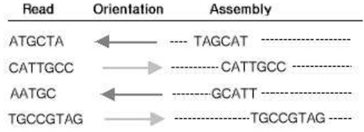
5. Unknown orientation. It is not known from which strand each fragment originates. This increases the complexity of the assembly task. Hence, a read may represent one strand or the reverse complement sequence on the other strand. A BAC-sized project may contain over 2000 reads and since it is not known from which strand each read originates, a duplicate, complementary set of reads is created by first reversing the base sequence and complementing each base. This results in a total of over 4000 reads (Figure 2.).

6. Polymorphisms. Complicates separation of nearly identical repeats. Polymorphisms will not usually be detected through “clone by clone” sequencing since only one variant for each genomic region is sampled.

7. Incomplete coverage. Coverage varies in different target sequence locations due to the nature of random sampling. The coverage has theoretically a certain probability to be zero depending on the average sampling coverage of the target genome, see equation 1. The number of gaps are further increased by bias due to the composition of the genomic sequence, e.g. some sequences may be toxic and interfere with the biology of the host organism.

3.3 Base calling

Commercial companies, such as Applied Biosystems that among other things produces DNA sequencers, have not made their algorithms public. However, public research for base calling on fluorescent data has been performed. Phred (Ewing et al., 1998) is today a popular base calling system that has challenged the ABI base calling. Tibbet, Bowling, and Golden(Adams et al., 1994) have studied base calling using neural networks and Giddings et al. (Giddings et al., 1993) describe a system that uses an object-oriented filtering system. Also, Dirk Walther et al. (Walther et al., 2001) describe a base calling algorithm reporting lower error rates than Phred.

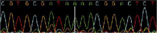
Base-calling refers to the conversion of raw chromatogram data into the actual sequence of bases figure 3. Using the Sanger sequencing method, extension reactions are performed using cloned or PCR product DNA segments as templates. The extensions generate products of all lengths as determined by the sequence. When these products are run on an electrophoresis gel, the base sequence can be read starting from the bottom. Different bases can be identified by labelling each base reaction with a different fluorescent dye. In sequencing machines using slab-gel or capillary technique, the dyes are exited with laser and the emitted light intensity is usually detected by a CCD-camera or a photo multiplier tube. This produces a set of four arrays called traces corresponding to signal intensities of each color over a time line. These traces are further processed by mobility correction, locating start and stop positions, base line substraction, spectral separation, and resolution enhancement. Base calling refers to the process of translating the processed data into an actual nucleotide sequence.

3.4 The Data Quality

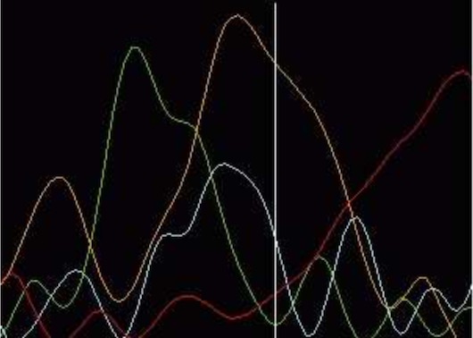
The limitation in current sequencing technology results in varying quality of the sequencing data between reads and within each read. In general the quality is lower towards the ends. There are number of reasons for this. The data at the end of the reads originates from the longest fragments and the proportional difference between long DNA fragments, differing only one base, is smaller than of that compared to short fragments. Also the random incorporation of ddNTPs results in a geometric distribution of concentration and size yielding a weaker fluorescent signal. Then there is the time factor. Molecules diffuse in the gel and the longer the time until the fragments pass the laser detector more they diffuse. These factors among others effectively prevent considerably longer reads than approximately one kilobase. In routine production the read length varies from about 400 bases to 800 bases. The sequence reads may also have low quality regions in the middle of high quality regions. These are mainly caused by the characteristics of polymerase and sequencing reactions. The base sequence of DNA itself has influence on the data quality. Single stranded DNA can self anneal to form a hair pin loop structure which causes it to move faster on the gel than would be expected according to its length. This is a fairly common phenomena on GC-rich segments and results in compression of trace peaks. Figure 4. Considering the

3.5 Error Probabilities

There are several obvious reason for why we would want to have error free sequence data. The fragment assembly problem would be algorithmically much simpler and the significantly lower cost associated with sequencing since fewer reads would be needed. Unfortunately, we cannot get perfect data, but we have to settle with the second best and try to measure the accuracy. In fact, many early base calling algorithms estimated confidence values (Giddings et al., 1993; Giddings et al., 1998; Golden et al., 1993) which is best done by studying electropherogram data. In 1994 Lawrence and Solovyev (Lawrence & Solovyev, 1994) carried out an extensive study defining a large number of trace parameters and an analysis to determine which ones are most effective in distinguishing accurate base calls. After 1998 when Brent Ewing and Phil Green implemented Phred (Ewing & Green, 1998), a base-calling program with the ability to estimate a probability of a basecall, Phred became one the most widely used base-calling programs today and Pred quality values became a standard within the sequencing community (P.Richerich, 1998). These quality values are logarithmic and range from 0 to 99 where increased value indicates increased quality. They are defined as follows: \[ q = −10 \cdot lg P \] Where q is the quality and P is the estimated error probability of a base-call. Phred quality values have a wide range. For example, a quality value 10 means that the probability of a base being wrong is \(\frac{1}{10}\) or having a 90% accuracy. An 99.99% accuracy is required for finished WGS data submitted into data bases, which means that the probability of an error is \( \frac{1}{1000} \).

Now we know that the root of many of the problems in fragment assembly essentially lies in the error prone base-calling. Ideally peaks in all four traces, one for each base, would be Gaussian-shaped with even distances without any background. As always in real life, several factors disturb the obtainable data quality, resulting in variable peak spacing, uneven peak heights and variable background. Thus, resulting in erroneous final nucleotide sequence. One of the key essences in successfull definition predictive error probabilities is the correct characterization of traces. Lawrence and Solovyev (Lawrence & Solovyev, 1994) considered single peaks in traces, but according to the work by Ewing and Green (Ewing & Green, 1998), the measures become more reliable when peaks in the neighborhood are taken into account. More information is available since indications of error may be present in near-by peaks but not in the peak under consideration. Ewing and Green found the following parameters to be the most important to effectively detect errors in base-calling:

1. Peak spacing, D. The ratio of the largest peak-to-peak distance, L_max to the smallest peak-to-peak distance, L_min, D = L_max . Computed in a window of L_min seven peaks which is centered on the current peak. This value measures the deviation from the ideal when peaks are evenly spaced, yielding a minimum value of one.

2. Uncalled/called ratio in window of seven peaks. The ratio of the amplitude of the largest peak not resulting in a base call to the amplitude of the smallest peak resulting in a base call, i.e. called peak. If the current window lacks an uncalled peak, the largest of the three remaining trace array values at the location of the called peak is used instead. In case the called base is an ’N’, phred vill assign a value of 100.0. The minimum value is 0 for traces with no uncalled peaks. With good data one of the four fluorscent signals will clearly dominate over the three other signals. Computed in a window of seven peaks centered at the base of interest.

3. Uncalled/called ratio in window of three peaks. The same as above, but using a window of three peaks.

4. Peak resolution. The number of bases between the current base and the nearest unresolved base. Base calls tend to be more accurate if the peaks are well separated and thus do not overlap significantly.

By re-sequencing an already known DNA sequence and using it as a golden standard, it is possible to compare the output of a base-caller program to this standard. The errors can now be categorized using the parameter values computed from the traces for each base. This can be used in predicting errors in unknown sequece by comparing the parameter values of the known errors frequencies. In order to compute new errors probabilities rapidly for unknown sequences, a lookup table is created where all four parameters values for each category of error rate is stored. Phred uses a lookup table consisting of 2011 lines to predict the error probability and to set the quality values.

The Phred quality values provide only information on the probability of a base being errorneously sequenced. Recall that there are four different types of errors that may occur in base-calling: substitutions, deletions, insertions and ambigous calls. Phred quality values do not give us a probability of a missing base, i.e. a probability of deletion. A recently published base-calling program, Life Trace by Dirk Walther et al. (Walther et al., 2001) introduces a new quality value, gap-quality. Pre-compiled versions of Life Trace for several different platforms are available at http://www.incyte.com/software/home.jsp.

The error probabilities can be used in several ways in fragment assembly programs. For example screening and trimming of reads and in defining pair-wise overlaps of reads. We discuss this more throughly in part 3.9

3.6 Genome Coverage

The benefit of the WGS method is that several reads usually cover the same region on both DNA strands and the a sought after consensus sequence can be computed using the information from several reads. Usually in a genomic sequencing project the coverage is about 8, often denoted as 8X. Coverage is defined as follows: \[ C = \frac{N \cdot r}{G} \] Where c = Coverage, N = Number of reads, r = Mean read length and G = Length of the genome. How many reads do we need to get 10X coverage of a BAC sequence of length 125 kb, if the mean read length is 480 bases? \[ N = \frac{c \cdot G}{r} = \frac{10 \times 125000}{480} = 2604 \: reads \] About 2600 fragments need to be sequenced to get 10X coverage. Remember that we don’t know the orientation of any of the fragments, therefore we need to complement all reads, i.e., compute the reverse complement sequence and then figure out the orientation in fragment assembly. This yields 2 · 2600 = 5200 reads, that an assembly program has to combat.

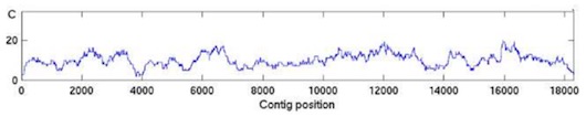
This is the total average coverage, but the actual observed coverage will vary along and between the assembled . The observed coverage is zero on regions that are not sequenced at all. Figure 5. shows a typical coverage variation along a which is sequenced using 10X average coverage.It may be valuable to know the probability to observe a coverage of certain depth or a resulting mean number of gaps and their average length. If we know the mean read length, r, average coverage, c and the length of the genomic region, G, the coverage can be computed using C as a binomial random variable. The WGS sequencing can be seen as randomly selecting an initial base as a starting position within the clone we aim to sequence and then continuing from that position forward an average read length number of bases. What is the probability of selecting this initial base? Let the average coverage be c = 8, the genome length G = 10⁴ bases and the average read length r = 500 bases. Using the equation (2), we can calculate that we have to sequence 1600 fragments to achieve the average coverage of 8. Thus, we will select a starting base for sequencing 1600 times, which gives us the probability of randomly selecting a base position, \[ p = \frac{No.\: of\: reads}{G} = \frac{1600}{10^{4}} = 0.016 \] Each selection or ’trial’ of a starting base results in ’success’ with the probability, p = 0.016 and in ’failure’, not selected with the probability 1 − p = 1 − 0.016 = 0.984. How many trials do we make? This may be a little tricky. The number of ’trials’ is the same as the average read length. We succeed to get one unit of coverage by selecting one of the positions in a window that equals the average read lengt. The probability of a succesful selection is p and the number of different ways we can select a base in the window is \( {r\choose c} \). If we think coverage C as the number c of “successes”, the probability to observe a certain coverage, C, can be computed using the binomial distribution function: \[ P\{C \leq i\} = \sum_{k=0}^{i}{r\choose k}p^{k}\left(1-p\right)^{r-k},\]\[ \: i = 0, 1, 2, ..., r \]

Example 1. Let coverage c = 8, the mean read length, r = 500 and the length of the clone, G = 10⁴. The probability of observing zero coverage, C is: \[ P\{C=0\} = 1 \times 1 \times \left( 1 - \frac{8}{500} \right)^{500}\] \[\approx 3.14 \times 10^{-4}, \] and the probability of observing a coverage, C = 12 is \[ P\{ C=12 \} = {500\choose 12} \left( \frac{8}{500}\right)^{12} \left( 1 - \frac{8}{500} \right)^{500-12}\] \[\approx 4.79 \times 10^{-2}, \] and the probability of a coverage, \(C ≤ 1\) is \[ P\{ C \leq 1 \} = P\{C=0\} + P\{C=1\} \] \[ 3.14 \times 10^{-4} + {500 \choose 1}\left( \frac{8}{500}\right)^{1} \left( 1 - \frac{8}{500} \right)^{500-1}\] \[\approx 2.56 \times 10^{-3} \] The Poisson random variable can be used to approximate the binomial random variable with parameters \( (n,p) \) when \(p\) is small and \(n\) large so that \(np\) is of moderate size. \(\lambda = np\)

The Poisson probability mass function: \[ p(i) = P\{ X=i \} = e^{-\lambda} \cdot \frac{\lambda^{i}}{i!} \]

The probability that a base is not sequenced: P₀ = e^−C , where C is the coverage. The total gap length = L X e^−C , average gap size = \(\frac{L}{n}\) , where n is the number n of randomly sequenced segments (Lander & Waterman, 1988; Fleischmann et al., 1995).

3.6.1 Exercises

1. Average coverage is 3.5, the mean read length 420 bases and the length of the BAC clone is 120 kb. Calculate the probability of a base not being sequenced.

2. Suppose you have a BAC sequence that contains two repeated regions of length 1 kb. The repeat copies differ 0.8% from each other and the mutations are evenly distibuted. You want that at least two differences are covered by at least four same reads with a porbability of 99.9%. What average coverage should you have?

3.7 Distance Constraints

When clones of DNA are sequenced from both ends, the approximate distance and their relative orientation is known. These sequence pairs from cloned ends are called mate-pairs (Myers et al., 2000) or sequence mapped gaps (Edwards & Caskey, 1990). The distance information can be used to both verify finished assemblies and as an additional source of information in assembly algorithms. The modified WGS sequencing strategy using these distance constraints is coined double-barreled. Typically a whole-genome sequencing projects use a mixture of clones containing inserts of several lengths, e.g. 2 kbp, 5 kbp, 50 kbp and 150 kbp clones. A usual way to employ the information in fragment assembly programs, is to build a so called scaffold. A scaffold is a set of or reads that are positioned, oriented and ordered corresponding to the distance information provided by cloned ends. Only an approximate length of clones are known and it is therefore not possible to rely only on one pair of cloned ends to build an assembly scaffold. To acquire a reasonable confidence, a certain coverage of mate-pairs is required. This is obviously dependent on the accuracy of the laboratory procedure when fragmented DNA seqments of a specific size are chosen. For example in the whole-genome WGS assembly of Drosophila, a single mate-pair information was found to be wrong 0.34% of the time, while two mate-pairs providing consistent information, the error was found to decrease to 10⁻¹⁵ (Myers et al., 2000).

3.8 Fragment Assembly Problem Models

The sequence reconstruction or fragment assembly problem would be easy if the original DNA sequence was unique, i.e. did not contain repeats. If we find a com- mon sub-sequence between two different reads 14 bases of length, the probability of finding an identical sequence by random is \( 4^{-14} = \frac{1}{268\:435\:456} \). This means 268 435 456 that if the length of the sequence we are assembling is about 270 Mbps, we would expect to find one such sequence by cheer chance. In a BAC-sized project ( 100000 bps) the probability of a random match is \( \frac{100\: 000}{268\:435\:456} \approx 4 * 10^{-4} \), the DNA sequence is random (NOTE that this is NOT the probability of two reads sharing a common sequence of a certain length). To solve the fragment assembly problem would be easy, since we would only need to find all the matching sub-sequences between all the reads and with a high probability almost all the overlaps assigned this way, would be correct. All what is left to do is to assemble these reads into contigous sequences, contigs, compute consensus sequence and we are done. Unfortunately, genomes usually are not random and contain repeats. This tactics is doomed to fail in practice.

During decades, many algorithms have been developed that attempt to solve the fragment assembly problem. One of the keys to good fragment assembly is a successful definition of overlaps between reads. These overlaps can be of four different types, Figure 6. Read A can overlap read B either at the

All fragments usually pass through a trimming process where low quality end are trimmed. If trimming is too stringent, information is lost and a greater number of reads is required to give a certain coverage. See section 3.6. On the other hand, if the trimming is too loose leaving many sequencing errors, it is difficult to determine whether the sequences come from the same region or if they just are very similar. Since many of the defined overlaps between reads are not right, it is very hard to rebuild the original genomic sequence. There will be extremely many ways to put this puzzle together. Actually so many ways, it is impossible to try out all the possibilities. It gives rise to a combinatorial explosion. This type of problem is very hard to solve and in computer science it is called non-deterministic polynomial complete, NP-complete. This is the hardest problem in NP. Thousands of problems have been proven to be NP-complete. One of the most famous is the Traveling Salesman Problem. Many computer scientists are working to find general solutions for this problem type. The simplest algorithm to solve this problem is the greedy algorithm.

3.8.1 The Shortest Common Superstring Model

The fragment assembly problem can be abstracted into the shortest common superstring problem (SCS). The object is to find the shortest possible superstring S that can be constructed from a given set of strings \(\tau\) so that \(S\) contains each string in \( \tau\) as a substring. SCS can also be be reduced to the traveling salesman problem and also has applications in data compression.

Maier and Storer showed that SCS is NP-complete (Maier & Storer, 1977). Later, in 1980, a more elegant proof was described (Gallant et al., 1980). Hence SCS is NP-complete, no feasible polynomial algorithm is known that solves this problem, but polynomial approximation algorithms exist. Moreover, SCS was proven to be MAX −SNP-hard in 1994 (Blum et al., 1994), meaning that no polynomial-time algorithm exists that can approximate the optimal solution within an arbitrary constant, but rather within a predetermined constant (section 3.1). A simple greedy algorithm can be used to approximate the solution by repeatedly choosing a maximum overlap between substrings in the set \(\tau \) until only one string is left. The greedy algorithm was first used in fragment assembly in 1979 (Staden, 1979).

Tarhio & Ukkonen and Turner established some performance guarantees for the greedy algorithm, which implied that the resulting superstring S is at most half the total, catenated length of the substrings in F (Tarhio & Ukkonen, 1988; Turner, 1989). Blum et al. were the first to describe an approximation algorithm for SCS with an upper bound of three times optimal (Blum et al., 1991). The approximation methods have been continuously refined. Kosaraju et al. established the bound of 250 (Kosaraju et al., 1994), Stein and Armen the bound of \( 2\frac{3}{4} \) in 1994 and \(2\frac{2}{3} \) bound in 1996 (Armen & Stein, 1994; Armen & Stein, 1996) and Sweedyk has reduced the bound to \(2 \frac{1}{2}\) (Sweedyk, 1995). It has been conjectured that greedy is at most two times optimal.

SCS is a sub-optimal model for fragment assembly, mainly because it tends to collapse repeated regions and it accounts for neither sequencing errors (i.e. sub- stitutions, insertions and deletions) nor unknown orientation.

3.8.2 The Sequence Reconstruction Model

The problem model derived from SCS that accounts for sequencing errors and for fragment orientation is called The Sequence Reconstruction Problem (SRP). The minimum number of edit operations, i.e. substitutions, insertions, deletions required to convert the sequence \(a\) into the sequence \(b\) is defined as the edit distance between sequences and denoted \(d(a, b)\). Given a set of sequence fragments, \( \tau \) and an sequencing error rate \( \epsilon \in [0,1] \), the object is to find the shortest sequence \(S\) such that for all \( f_{i} \in \tau \), there is a substring \(S_{sub}\) of \(S\) such that \[ min\{ d(S_{sub}, f_{i}), d(S_{sub}, f_{r}^{i}) \} \leq \epsilon |S_{sub} |, \] where \(f_{i}^{r}\) is the reverse complement of \(f_{i}\).

Since the sequence reconstruction problem can be reduced to NP-complete SCS with zero error rate, SRP is also NP-complete. The proof was given in 1996 (Waterman, 1996).

Peltola et al. (Peltola et al., 1984) were the first to include errors and fragment orientation in the problem model together with graph theory, and they used the greedy algorithm to approximate the fragment layout. Also, Huang included the error criterion in the CAP assembly program (Huang, 1992). Kececioglu and Myers describe the extension to SRP by introducing discrimination of false overlaps based on error likelihood including an extensive treatment of the unknown orientation problem using interval graphs (Kececioglu, 1991; Kececioglu & Myers, 1995). Phrap uses Phred quality values in a likelihood model to discriminate false overlaps (section 3.9.2 and 3.9.3).

The sequence reconstruction model complies better with the reality than the shortest common superstring model.

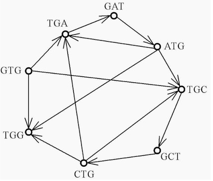
3.8.3 Graphs

An article by L. Euler started a branch of mathematics called graph theory (Euler, 1736; N. Biggs & Wilson, 1976). A graph is a collection of vertices connected by edges. Since each read should form an interval on the target sequence, it is natural to model this problem as an interval graph problem, with reads corresponding to vertices and overlaps to edges. The directed graph \( G_{ov}(V,E) \) in figure 8 for the sequence S = GTGATGCTGG has a vertex set V = GTG, TGA, GAT, ATG, TGC, GCT, CTG, TGG. Each edge E is an overlap with an adjacent sequence by the minimum of two bases. A Hamiltonian path in the graph is a path that passes through every vertex exactly once. However, a Hamiltonian path does not necessarily pass through all the edges. A Hamiltonian cycle or circuit is a Hamiltonian path that ends in the same vertex as that in which it started. Each edge in the graph can be weighted by a score that reflects the quality of an overlap and the traveling salesman problem formulation can be used to find the Hamiltonian path that yields the best score. This problem is however NP-complete. If the amount of input data is large, and in particular in the presence of similar repeats

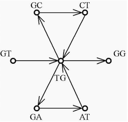
An alternate data structure can be used to find Euler paths. An Euler path in a graph is a path that travels along every edge exactly once, but might pass through individual vertices of the graph more than once. An Euler path that begins and ends in the same vertex is an Euler circuit or tour. The redundant WGS data can be converted into an Euler path problem by producing k-tuple data. This is done by extracting all overlapping k-tuples from all WGS reads and then collapsing all edges to single edges where data is consistent so that only unique k-tuples remain. The graph is constructed on (k − 1)-tuples so that each edge has a length of one. For each read fragment f of length k in S an edge from the vertex labeled with the left-most k − 1 bases of f is directed to the node labeled with the right-most k − 1 bases of f . Edges may be weighted by e.g. the number of fragments associated with an edge. An example of a directed graph \(G_{eu}\) is the case shown in figure 9, that is constructed for the sequence S with k = 3.

The fragment assembly problem is now recast into the problem of finding an Euler path in the graph and there are efficient algorithms for finding such paths. The reduction of sequencing by hybridization (SHB) to a question of finding Euler paths was originally developed by Pevzner (Pevzner, 1989) and the hybrid algorithm, based on SHB, was described by Idury and Waterman (Idury & Waterman, 1995). This problem is not NP-complete. However, this gain is paid partly by some loss of information in the process of fragmenting the original input data into a number of k-tuples. There may be several Euler paths in one graph, as shown in figure 9, that start at the vertex labeled GT and results in the sequences shown in figure 10.

One approach of getting the set of all Euler paths in a graph is based on the fact that all spanning trees can be enumerated and that there is a relationship between the set of all spanning trees and the set of all Euler paths in a graph (Even, 1979). Another approach is to transform any compatible string by a series

The Euler path method produces single sequences as output. A multiple alignment is required to evaluate the underlying read data. This can be accomplished by aligning all the initial reads against the Euler sequence(s).

Idealized versions of problem models are rarely applicable in practice. Sequencing errors, in particular together with nearly identical repeats, are a complicating factor. Overlaps are based on exact sequence identity, thus there is a possibility of losing existing overlaps because the identities are distorted by sequencing errors. The input data may be trimmed to be of very high quality, yet this results in shorter read lengths. However, it is possible to try to correct the errors prior to the construction of the graph, as is the approach used in the EULER assembler (Pevzner et al., 2001).

The Euler path method produces single sequences as output. A multiple alignment is required to evaluate the underlying read data. This can be accomplished by aligning all the initial reads against the Euler sequence(s).

Idealized versions of problem models are rarely applicable in practice. Sequencing errors, in particular together with nearly identical repeats, are a complicating factor. Overlaps are based on exact sequence identity, thus there is a possibility of losing existing overlaps because the identities are distorted by sequencing errors. The input data may be trimmed to be of very high quality, yet this results in shorter read lengths. However, it is possible to try to correct the errors prior to the construction of the graph, as is the approach used in the EULER assembler (Pevzner et al., 2001).

3.9 Algorithms

The fragment reconstruction problem based on overlaps can in turn be divided into a number of sub-problems. 1. Discarding contamination, i.e. sequences from vector and chimeric reads and the host organism. 2. Determination of all overlaps between reads. 3. Computation of the layout of the contigs, i.e. the orientation and relative position of the reads in contigs. 4. Creation of multiple alignments of all reads. 5. Computation of the consensus sequences.

3.9.1 Contamination

Contaminating reads can easily be discarded by screening the reads against a database consisting of the host genome sequences, as well as the vector sequences. Since chimeric reads are composites, consisting of at least two sequences originating from different locations of the target genome, they can be recognized by their pattern of overlap with other reads. One such algorithm was described in 1996 and implemented in CAP2 (Huang, 1996).

3.9.2 Overlap Detection

In order to determine all pairwise overlaps, an all-versus-all comparison of reads has to be performed. For example, 2,000 reads would require \( (2 \cdot 2000)^{2} \) = 16,000,000 pair-wise comparisons, since each possible orientation is tested. The classical solution to this problem of approximate string matching is a dynamic programming method (Sellers, 1980). The disadvantage of this approach is the quadratic running time, O(nm), where n and m are the lengths of the reads. There are several approaches that improve the running time by only computing a part of the dynamic programming matrix, for example Ukkonen who reduces the time to O(nk), where k is the edit distance (Ukkonen, 1985). The performance can be further improved by pre-prossessing the database using indexing techniques, such as patricia trees (Knuth, 1973), suffix trees (McCreight, 1976) and suffix arrays (Manber et al., 1990). These structures allow a query time proportional to the length of the query string, while being independent of the size of the database, which can be contructed in linear time. The time to construct the database can be amortized by performing a large number of queries.

There are many different approaches to solving the all-versus-all comparison problem (Gusfield, 1997; Chen & Skiena, 1997). One solution that was used in the TIGR Assembler, was to locate all k-tuples shared between read pairs, similar to the initial processing in BLAST (Altschul et al., 1990). A more practical solution, that can be applied to WGS reads, is to use a combination of suffix arrays and indexes built of the database sequences (Myers, 1995a). A suffix array can be constructed by indexing all instances of short words, typically 10 to 14 bases, that occur in the database. All instances of words are stored in an array. By assigning pointers to point to their locations in reads, the lists of suffixes in each array position can be sorted in lexicographical order. In this way, all similar reads will be grouped close to each other and it is possible to rapidly extract matching suffixes. The candidate alignments are created by dynamic programming, where only a band in the dynamic programming matrix is computed (Chao et al., 1992), or a variation of the Smith-Waterman algorithm (SWA) (Smith & Waterman, 1981) is used. This method is used in the Phrap fragment assembly program and similar methods with some variation are used in many other assembly programs, e.g. in FALCON (Gryan, 1994) and ARACHNE (Batzoglou et al., 2002). Approaches based on hybridization and techniques based on the sampling of large numbers of segments, sub-words (Kim & Segre, 1999), have not yet been shown to be successful in practice, mainly due to the presence of ubiquitous repeats. Each of the pair-wise alignments are scored in order to evaluate the quality of overlaps. The total score is obtained by dynamic programming using a scoring scheme with specified match score, and using mismatch and gap penalties (Pearson & Lipman, 1988; Altschul et al., 1990), possibly together with some estimate of the total sequencing error, as in the assembly programs, CAP and CAP2 (Huang, 1992; Huang, 1996). A more accurate approach is to utilize quality values, i.e. the probability that a base is erroneously called. Most fragment assembly programs that use error probabilities, use quality values generated by Phred, which is the most widely used base calling program. Several programs use the error probabilities merely as weights for match score, mismatch and gap penalties, e.g. STROLL (Chen & Skiena, 2000) and CAP (Huang & Madan, 1999). Phrap uses Phred quality values in a likelihood model to discriminate false overlaps. The initial candidate overlaps are initially filtered by a minimum SWA score and then all alignments are re-scored by computing a log likelihood ratio (LLR), which is used in the construction of contigs.

The pair-wise overlaps can be used to generate overlap graphs, where each read and its reverse complement are nodes and edges represent the overlaps between reads. Edges are weighted by some measure that reflects the strength of an overlap, such as pair-wise alignments scores combined with the lengths of clone inserts.

3.9.3 Contig Layout Determination

The problem of creating the fragment layout in contigs, i.e. the problem of de- termining the relative order and offset of all reads, is based on the reconstruction model and is NP-complete (Gallant et al., 1980; Gallant, 1983; Kececioglu, 1991). Hence, all methods rely mostly on heuristics to combine reads. Several sophis- ticated methods to approximate the optimal solution have been described, for example, relaxation based on sorting overlaps by decreasing score or spanning forests (Kececioglu, 1991), methods based on simulated annealing (Burks et al., 1994), reduction to greedy Eulerian tour (see section 3.8.3), using genetic algo- rithms (Parsons & E., 1995) or by a series of reductions to an overlap graph that reduce the number of edges and vertices without changing the space of potential solutions (Myers, 1995b).

Most of the approximation algorithms perform well on non-repeated data, but have trouble with the determination of the correct layout in the presence of repeats. This is true in particular when repeats are highly similar and longer than the average read length. In order to avoid confusing assembly algorithms, several assembly strategies screen for repeats in the input data set against a database prior to assembly in order to assemble reads originating from non-repeated regions of the target sequence into a number of contigs. These contigs may then be ordered using clone length constraints given by the sequencing of both ends of clone inserts. This is the approach used in the Celera Assembler (Anson & Myers, 1999; Myers et al., 2000; Huson et al., 2002). This leaves most of the long repeated regions unordered. Other ways to detect reads originating from repeated regions of the target sequence are the computation of a probability of observed coverage, which is not a precise method, and the detection of conflicting paths in an overlap graph (Myers, 1995b).

Phrap uses the greedy method, in which the overlaps are first sorted by their LLR-scores and are joined together into contigs in descending LLR-score order. Additional information, such as coverage on both strands are used to confirm read positions. Moreover, the layout may be broken at weak overlaps and the layout recomputed. The sequencing from both ends of an insert yields distance constraints that can be used both to confirm an assembly, and to aid in the ordering of the pair-wise overlaps e.g. the TIGR Assembler, CAP3 and ARACHNE, as well as in the Celera Assembler.

3.9.4 Creation of Multiple Alignments

In order to get the final result, the consensus sequence, a multiple alignment of the reads in each contig has to be computed. There are several multiple alignment methods, that differ mostly by the criteria for selecting pairs of alignments and thereby the order in which pairs are merged (Gusfield, 1997). However, WGS read fragments that are aligned into a contig are assumed to represent the same region of the target sequence. Therefore the global alignments are most commonly created by the simple approach of repeatedly aligning the next read with the cur- rent alignment, as for example in CAP3. This simple approach results in multiple alignments that are not locally optimized. In most cases, local deviations in the multiple alignments will only have a small effect on the quality of the computed consensus sequence. The multiple alignments can be locally optimized by an algo- rithm described by Anson and Myers, where each sequence is iteratively aligned to a consensus structure (Anson & Myers, 1997). After each round of alignments, the score is computed and compared to the previous score. The iterations are continued until no lower score can be obtained.

3.9.5 Computation of the Consensus Sequence

The consensus sequence can be computed using simple majority voting. When quality values for bases are available, more sophisticated methods may be applied. The scheme used in CAP3 assumes that the errors are independently distributed between the strands. For each column of the alignment the quality values for the base types are partitioned into two groups, one from each strand. The quality values in each group are sorted in decreasing order and the highest quality value in each group is given the weight of 1.0 and the rest the weight of 0.5. The sum of quality values is computed. The base with the largest quality value is taken as the consensus base for the column and the quality of the consensus base is the sum of quality values for every base minus the sum of the quality values for the other bases.

Phrap uses an approach where an interval of the best quality read is chosen to represent the consensus sequence of that interval of the multiple alignment. A weighted directed graph, where the nodes represent selected read positions and the bidirectional edges, that represent aligned positions in two overlapping reads with the weight of zero, is constructed. In addition, the undirectional edges between positions in the same read with the weight of the sum of the quality values for the bases between the positions are used. The contig sequence is the path with the highest weight in the graph. Hence, the method used in Phrap does not yield a consensus sequence in the proper sense, but is instead a mosaic of the highest quality regions.

4 WGS Fragment Assembly Programs

4.1 Phrap

Several programs are needed to do complete assembly: phred (Ewing et al., 1998)(Ewing & Green, 1998) cross-match, repeat-masker, phrap (http://www.phrap.org) and consed (Gordon et al., 1998). Phred reads the trace files produced by a sequencing machine, does base calling and assigns quality values, i.e. error rates for each base. These quality values reflect the estimated probability that a base is errorneously called. Cross-match is useful in finding vector sequences in reads.

The assembly is performed by Phrap that uses the quality information provided by Phred (see section 3.5) to make pair-wise comparisons of reads. This method has the advantage that it can use almost the whole read length without any significant trimming, since low quality base calls can be ignored. Phrap makes use of the information provided by both DNA strands by assuming that the base calls are independent between the opposite strands. Phrap may confirm a base call by another call on the opposite strand by summing it with the score of the confirming call. The same is true for calls performed using different chemistries. Phrap uses the Phred quality scores to discriminate putative repeats by likelihood ratios. If mismatches occur along the alignment at positions where base qualities are high, they are assumed to be due to repeats and reads are not overlapped. If mismatches occur at low quality positions, they are assumed to be due to base calling errors.

RepeatMasker is a program developed to screen sequences for known repeats to avoid false overlaps due to repeated regions in the sequenced genomic region. Detected repeats are masked and not used during the assembly process.

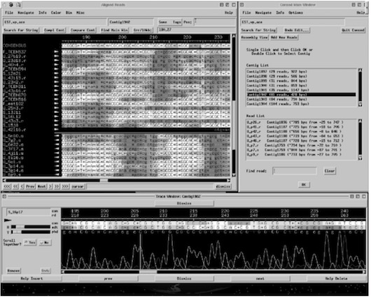
Phrap computes the final sequence or consensus sequence from sections of highest quality regions of the reads in assembled contigs. Consed is used to view the results of the assembly. Figure 11. shows a screen shot of Consed.

4.1.1 The Phrap Method

The hardest step in the assembly process is to determine the correct pattern of how all the reads align relative to each other (layout). Phrap uses the greedy algorithm together with log likelihood ratios, LLR scores for overlaps, to determine the layout of reads. LLR scores are computed using Phred quality values or error probabilities. The sum of LLR scores are then used to decide if discrepancies in overlaps are real, or if they are due to base-calling errors.

Candidate overlaps are obtained by dynamic programming and scored initially without quality values. The scores for these candidate overlaps are re-computed using error probabilities. The log likelihood ratio H₁/H₀ is computed for each base pair in an overlap and the score of the overlap is the sum of the LLR scores for each base pair. H₁: the probability of observed data assuming overlap is real. H₀: the probability observing the data assuming reads are from 95% similar repeats. The figure 95% is found to work well in practice.

Following assumptions are made:

1. Alignment positions are independent of each other

2. When a base-calling error occurs at a read position, the base calls in the two reads disagree at the position. (Correction required to avoid this assumption is very small).

3. Errors in reads are independent of each other.

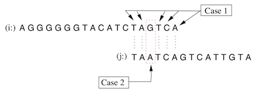
The base pairs in an alignment may match or mismatch. This yields two cases if possible insertions and deletions are not counted.

Case 1: Bases match. \[ Prob(agree|H_{1}(overlap)) =\]\[ (1-p_{i})(1-p_{j}) \] \[ Prob(agree|H_{0}(repeat)) =\] \[(1 - p_{i})(1 - p_{j}) * 0.95 \] \[ LLR = log Left( \frac{1}{0.95} right) \]

Case 2: Discrepancy between base cells: \[ Prob(discrep|H_{1}(overlap)) =\] \[p_{i} + p_{j} − p_{i} \cdot p_{j} \] \[ Prob(discrep|H_{0}(repeat)) =\] \[0.05 + 0.95(p_{i} + p_{j} − p_{i} \cdot p_{j}) \] \[ LLR \approx \log \left( \frac{0.05+0.95(p_{i} +p_{j} −p_{i} \cdot p_{j})} {p_{i} + p_{j} − p_{i} \cdot p_{j}} \right) \] Where p_i = probability that the base in sequence i is errorneous and p_j = probability that the base in sequence j is errorneous. See figure 12.

4.1.2 Greedy Algorithm for Layout Construction

Once all overlaps between reads are computed, the layout, or the order of how the reads align realitive to each other, can be determined. Phrap maintains the layout of reads in a graph, where the orientation and offset with respect to the start of a contig is stored. Vertices in this graph represent reads and edges represent overlaps. Thus, a contig is the connected component in the graph.

Reads are added to a contig using the greedy algorithm. Initially, each read forms a separate contig. Each read pair is then processed in decreasing LLR score order. Each time a read pair is chosen, a potential merge between different contigs is considered. No negatively scoring read pairs are allowed into a contig and read pairs must have consistent offset in the candidate contig.

The greedy algorithm together with LLR scores will always result in average correct assemblies. Phrap enchances this result by breaking the layout in positions where reads have positive scores in alternative locations. This time an exhausting computation is performed, i.e. all possible ways of joining the read fragments is considered and the highest scoring alternative is chosen.

4.1.3 Construction of Contig Sequences

The final sequence is not strictly a consensus sequence, since the contig sequence is constructed from the highest quality regions of the reads. The comlumn positions in a contig are never evaluated. The main steps are as follows:

1. Construct a weighted directed graph:
- Nodes are selected read positions.
- Edges are of two types: 1) Bidirectional: These edges are between aligned positions in two overlapping reads. The weights of the edges are zero. 2) Undirectional: These are between positions in the same read in the 3’ to 5’ direction. Weight of these edges is the sum of Phred quality measures for bases.

2. Determine the contig sequence from the read segments that lie on the highest weight path through the graph. The highest weight path can be obtained using Tarjan’s algorithm with modifications to deal with non-trivial cycles.

Bioinformatics Education and Tutorials

Learn fundamental and advanced topics in bioinformatics. Continually updated.

View

History of computing and genetics

Roots and development of the field of bioinformatics.

View

Science Blogs

A wide range of articles within bioinformatics, genetics, and related fields. We write new materials every week.

View

Software

Software tools are supporting tutorials. For example, Analysis of DNA alignment scoring, make any PAM scoring matrix, and other tools.

View

References

Adams, M., Celniker, S., Holt, R., Evans, C., Gocayne, J., Amanatides, P., Scherer, S., Li, P., Hoskins, R., Galle, R., George, R., Lewis, S., Richards, S., Ashburner, M., Henderson, S., Sutton, G., Wortman, J., Yandell, M., Zhang, Q., Chen, L., Brandon, R., Rogers, Y., Blazej, R., Champe, M., Pfeiffer, B., Wan, K., Doyle, C., Baxter, E., Helt, G., Nelson, C., Gabor, G., Abril, J., Agbayani, A., An, H., Andrews-Pfannkoch, C., Baldwin, D., Ballew, R., Basu, A., Baxendale, J., Bayraktaroglu, L., Beasley, E., Beeson, K., Benos, P., Berman, B., Bhandari, D., Bolshakov, S., Borkova, D., Botchan, M., Bouck, J., Brokstein, P., Brottier, P., Burtis, K., Busam, D., Butler, H., Cadieu, E., Center, A., Chandra, I., Cherry, J., Cawley, S., Dahlke, C., Davenport, L., Davies, P., de Pablos, B., Delcher, A., Deng, Z., Mays, A., Dew, I., Dietz, S., Dodson, K., Doup, L., Downes, M., Dugan-Rocha, S., Dunkov, B., Dunn, P., Durbin, K., Evangelista, C., Ferraz, C., Ferriera, S., Fleischmann, W., Fosler, C., Gabrielian, A., Garg, N., Gelbart, W., Glasser, K., Glodek, A., Gong, F., Gorrell, J., Gu, Z., Guan, P., Harris, M., Harris, N., Harvey, D., Heiman, T., Hernandez, J., Houck, J., Hostin, D., Houston, K., Howland, T., Wei, M., Ibegwam, C., Jalali, M., Kalush, F., Karpen, G., Ke, Z., Kennison, J., Ketchum, K., Kimmel, B., Kodira, C., Kraft, C., Kravitz, S., Kulp, D., Lai, Z., Lasko, P., Lei, Y., Levitsky, A., Li, J., Li, Z., Liang, Y., Lin, X., Liu, X.,Mattei, B., McIntosh, T., McLeod, M., McPherson, D., Merkulov, G., Mil- shina, N., Mobarry, C., Morris, J., Moshrefi, A., Mount, S., Moy, M., Murphy, B., Murphy, L., Muzny, D., Nelson, D., Nelson, D., Nelson, K., Nixon, K., Nusskern, D., Pacleb, J., Palazzolo, M., Pittman, G., Pan, S., Pollard, J., Puri, V., Reese, M., Reinert, K., Remington, K., Saunders, R., Scheeler, F., Shen, H., Shue, B., Siden-Kiamos, I., Simpson, M., Skupski, M., Smith, T., Spier, E., Spradling, A., Stapleton, M., Strong, R., Sun, E., Svirskas, R., Tec- tor, C., Turner, R., Venter, E., Wang, A., Wang, X., Wang, Z., Wassarman, D., Weinstock, G., Weissenbach, J., Williams, S., Woodage, T., Worley, K., Wu, D., Yang, S., Yao, Q., Ye, J., Yeh, R., Zaveri, J., Zhan, M., Zhang, G., Zhao, Q., Zheng, L., Zheng, X., Zhong, F., Zhong, W., Zhou, X., Zhu, S., Zhu, X., Smith, H., Gibbs, R., Myers, E., Rubin, G. & Venter, J. (2000) The genome sequence of drosophila melanogaster. Science, 287 (5461), 2185–95. PubMed

Adams, M., Fields, C. & Venter, J., eds (1994) Neural networks for automated basecalling of gel-based DNA sequencing ladders. Academic Press, San Diego, CA.

Allison, D., Thompson, J., Jacobson, K., Warmack, R. & Ferrel, T. (1990) Scanning tunneling microscopy and spectroscopy of plasmid DNA. Scanning Microscience, 4, 517–522.

Altschul, S., Gish, W., Miller, W., Myers, E. & Lipman, D. (1990) Basic local alignment search tool. J. Mol. Biol., 215 (3), 403–10. PubMed

Anderson, S. (1981) WGS DNA sequencing using cloned DNase I-generated fragments. Nucleic Acids Res., 9 (13), 3015–27. PubMed

Anderson, S., Bankier, A., Barrell, B., de Bruijn, M., Coulson, A., Drouin, J., Eperon, I., Nierlich, D., Roe, B., Sanger, F., Schreier, P., Smith, A., Staden, R. & Young, I. (1981) Sequence and organization of the human mitochondrial genome. Nature, 290 (5806), 457–65. PubMed

Anson, E. & Myers, E. (1997) Realigner: a program for refining DNA sequence multialignments. J. Comp. Biol., 4 (3), 369–383. PubMed

Anson, E. & Myers, G. (1999) Algorithms for whole genome WGS sequencing. In Proc. RECOMB ’99 pp. 1–9, Lyon, France.

Armen, C. & Stein, C. (1994). In A 2.75 approximation algorithm for the shortest superstring problem DIMACS Workshop on Sequencing and Mapping.

Armen, C. & Stein, C. (1996) A 2 2/3-approximation algorithm for the shortest superstring problem. In Combinatorial Pattern Matching pp. 87–101. Springer

Baer, R., Bankier, A., Biggin, M., Deininger, P., Farrell, P., Gibson, T., Hatfull, G., Hudson, G., Satchwell, S., C, C. S., Tuffnell, P. & Barrell, B. (1984) DNA sequence and expression of the B95-8 Epstein-Barr virus genome. Nature, 310 (5974), 207–11. Nature

Batzoglou, S., Berger, B., Mesirov, J. & Lander, E. S. (1999) Sequencing a genome by walking with clone-end sequences: a mathematical analysis. Genome Re- search, 9 (12), 1163–74. PubMed

Batzoglou, S., Jaffe, D. B., Stanley, K., Butler, J., Gnerre, S., Mauceli, E., Berger, B., Mesirov, J. P. & Lander, E. S. (2002) ARACHNE: a whole–genome WGS assembler. Genome Research, 12, 177–189. PubMed

Benzer, S. (1959) On the topology of the genetic fine structure. Proc. Natl. Acad. Sci., 45, 1607–1620. PMC

Bernal, A., Ear, U. & Kyrpides, N. (2001) Genomes online database (GOLD): a monitor of genome projects world–wide. Nucleic Acids Res., 29 (1), 126–127. PubMed

Blattner, F. R., III, G. P., Bloch, C. A., Perna, N. T., Burland, V., Riley, M., Collado-Vides, J., Glasner, J. D., Rode, C. K., Mayhew, G. F., Gregor, J., Davis, N. W., Kirkpatrick, H. A., Goeden, M. A., Rose, D. J., Mau, B. & Shao, Y. (1997) The complete genome sequence of Escherichia coli K–12. Science, 277 (5331), 1453–74. PubMed

Blum, Avrim, Jiang, T., Li, M., Tromp, J. & Yannakakis, M. (1991) Linear approxmation of shortest superstrings. In Proceedings of the 23rd AC Symposium on Theory of Computation pp. 328–336.

Blum, A., Jiang, T., Li, M., Tromp, J. & Yannakis, M. (1994) Linear approximation of shortest superstrings. J. of the ACM, 41, 634–47.

Bonfield, J., Smith, K. & Staden, R. (1995) A new DNA sequence assembly program. Nucleic Acids Res., 23 (24), 4992–9. PubMed

Bonfield, J. & Staden, R. (1995) The application of numerical estimates of base calling accuracy to DNA sequencing projects. Nucleic Acids Res., 23, 1406– 1410. PubMed

Brenner, S., Johnson, M., Bridgham, J., Golda, G., Lloyd, D., Johnson, D., Luo, S., McCurdy, S., Foy, M., Ewan, M., Roth, R., George, D., Eletr, S., Albrecht, G., Vermaas, E., Williams, S., Moon, K., Burcham, T., Pallas, M., DuBridge, R., Kirchner, J., Fearon, K., Mao, J. & Corcoran, K. (2000a) Gene expression analysis by massively parallel signature sequencing (mpss) on microbead arrays. Nat. Biotechnol., 18 (6), 630–4. PubMed

Brenner, S., S.R.Williams, Vermaas, E., Storck, T., Moon, K., McCollum, C., Mao, J., Luo, S., Kirchner, J., Eletr, S., DuBridge, R., Burcham, T. & Albrecht, G. (2000b) In vitro cloning of complex mixtures of DNA on microbeads: physical separation of differentially expressed cDNAs. Proc. Natl. Acad. Sci., 97 (4), 1665–70. PubMed

Burks, C., Engle, M., Forrest, S., Parsons, R., Soderlund, C. & Stolorz, P. (1994) Automated DNA Sequencing and Analysis. Academic Press, New York pp. 249–259.

C. Elegans Sequencing Consortium (1998) Genome sequence of the nematode C. elegans: A platform for investigating biology. Science, 282, 2012–2018. PubMed

Chao, K., Pearson, W. & Miller, W. (1992) Aligning two sequences within a specified diagonal band. Comput. Appl. Biosci., 8 (5), 481–7. PubMed

Cheeseman, P., Kanefsky, B. & Taylor, W. M. (1991) Where the Really Hard Problems Are. In Proceedings of the Twelfth International Joint Conference on Artificial Intelligence, IJCAI-91, Sidney, Australia pp. 331–337. PDF

Chen, E., Schlessinger, D. & Kere, J. (1993) Ordered WGS sequencing, a strategy for integrated mapping and sequencing of YAC clones. Genomics, 17, 651–656. PubMed

Chen, T. & Skiena, S. (1997) Trie–based data structures for sequence assembly. In The Eight Symbosium on Combinatorial Pattern Matching pp. 206–223. ACM

Chen, T. & Skiena, S. S. (2000) A case study in genome–level fragment assembly. Bioinformatics, 16 (6), 494–500. PubMed

Chen, W. & Hunkapiller, T. (1992) Sequence accuracy of large DNA sequencing projects. DNA Sequence – Journal of DNA Sequences and Mapping, 2, 335– 342. PubMed

Churchill, G. & Waterman, M. (1992) The accuracy of DNA sequences: estimating sequence quality. Genomics, 14, 89–98. PubMed

Clarke, L. & Carbon, J. (1976) A colony bank containing synthetic ColE1 hybrid plasmids representative of the entire E. coli genome. Cell, 9, 91–101. PubMed

Cook, S. (1971) The complexity of theorem-proving procedures. In Proc. 3rd Ann. ACM Symp. on Theory of Computing pp. 151–158.

Dayhoff, M. (1964) Computer aids to protein sequence determination. J. Theor. Biol., 8, 97–112.

Dear, S. & Staden, R. (1991) A sequence assembly and editing program for efficient management of large projects. Nucleic Acid Res., 19, 3907–3911. PubMed

Deininger, P. (1983) Approaches to rapid DNA sequence analysis. Anal. Biochem., 135 (2), 247–63.

Drmanac, R., Labat, I., Brukner, I. & Crkvenjakov, R. (1989) Sequencing of megabase plus DNA by hybridisation: theory of the method. Genomics, 4, 114–128. scienceDirect

Edwards, A. & Caskey, C. (1991) Closure Strategies for Random DNA Sequencing. Methods: A Companion to Methods in Enzymology, 3, 41–47. scienceDirect

Eichler, E. (1998) Masquerading repeats: paralogous pitfalls of the human genome. Genome Research, 8, 758–762. Genome Research

Euler, L. (1736) Solutio problematis ad geometriam situs pertinentis. Commenrarii Academiae Scientiarum Imperialis Petropolitanae, 8, 128–140.

Even, S. (1979) Graph Algorithms. Computer Science Press, Mill Valley, CA.

Ewing, B. & Green, P. (1998) Base-calling of automated sequencer traces using phred. ii. error probabilities. Genome Research, 8, 186–194. PubMed

Ewing, B., Hillier, L., Wendl, M. & Green, P. (1998) Base-calling of automated sequencer traces using Phred I. Accuracy Assessment. Genome Research, 8, 175–185. PubMed

Fleischmann, R., Adams, M., White, O., Clayton, R., Kirkness, E. & Kerlavage, A. (1995) Whole-genome random sequencing and assembly of haemophilus influenzae rd. Science, 269, 496–512. PubMed

Fuhrman, S., Deininger, P., LaPorte, P., Friedmann, T. & Geiduschek, E. (1981) Analysis of transcription of the human Alu family ubiquitous repeating element by eukaryotic RNA polymerase III. Nucleic Acids Res., 9 (23), 6439–56. Nucleic Acids Res.

Gallant, J. (1983) The complexity of the overlap method for sequencing biopolymers. Journal of Theoretical Biology, 101, 1–17. Europe PMC

Gallant, J., Maier, D. & Storer, J. (1980) On finding minimal length superstrings. Journal of Computer and System Sciences, 20, 50–58. PDF (core.ac.uk)

Garey, M. R. & Johnson, D. S. (1979) Computers and Intractability: A Guide to the Theory of NP-Completeness. Freeman, New York.

Giddings, M., Jr., R. B., Haker, M. & Smith, L. (1993) An adaptive, object oriented strategy for base calling in DNA sequence analysis. Nucleic Acids Res., 21, 4530–4540. PubMed

Giddings, M., Severin, J., Westphall, M., Wu, J. & Smith, L. (1998) A software system for data analysis in automated DNA sequencing. Genome Res., 8, 644–665. Genome Res.

Gingeras, T., Milazzo, J., Sciaky, D. & Roberts, R. (1979) Computer programs for the assembly of DNA sequences. Nucleic Acid Res., 7, 529–545 Nucleic Acid Res..

Goffeau, A., Barrell, B., Bussey, H., Davis, R., Dujon, B., Feldmann, H., Galibert, F., Hoheisel, J., Jacq, C. & Johnston, M. (1996) Life with 6000 genes. Science, 274 (546), 563–567. Science

Golden, J., Torgersen, D. & Tibbets, C. (1993) Pattern recognition for automated dna sequencing, i: on-line signal conditioning and feature extraction for basecalling. In Proceedings of the first International Conference on Intelligent Systems for Molecular Biology, (et al., L. H., ed.), AAAI Press, Menlo Park, CA.

Gordon, D., Abajian, C. & Green, P. (1998) Consed: a graphical tool for sequence finishing. Genome Research, 8, 195–202. Genome Research

Green, P. (1997) Against a whole–genome WGS. Genome Research, 7, 410–417. Genome Research

Gronenborn, B. & Messing, J. (1978) Methylation of single-stranded DNA in vitro introduces new restriction endonuclease cleavage sites. Nature, 272 (5651), 375–377. Nature

Gryan, G. (1994) Faster sequence assembly software for megabase WGS assem- blies. In Genome Sequencing and Analysis Conference VI.

Gusfield, D. (1997) Algorithms on strings, trees, and sequences: computer science and computational biology. Press Syndicate of the University of Cambridge, New York, NY.

Holley, R. W., Apgar, J., Everett, G. A., Madison, J. T., Marquisee, M., Merrill, S. H., Penswick, J. R. & Zamir, A. (1965) Structure of a ribonucleic acid. Science, 147, 1462–1465. Science

Huang, X. (1992) A contig assembly program based on sensitive detection of fragment overlaps. Genomics, 14, 18–25. PubMed

Huang, X. (1996) An improved sequence assembly program. Genomics, 33, 21–31. PubMed

Huang, X. & Madan, A. (1999) CAP3: a DNA sequence assembly program. Genome Research, 9, 868–877. PubMed

Huson, D., Reinert, K. & Myers, E. (2002). The greedy path–merging algorithm for sequence assembly. J. Comp. Biol. MyersLab - PDF

Hutchinson, G. (1969) Evaluation of polymer sequence fragment data using graph theory. Bulletin of Mathematical Biophysics, 31, 541–562. Springer

Idury, R. & Waterman, M. (1995) A new algorithm for WGS sequencing. J. Comp. Biol., 2, 291–306. PubMed

Karas, M. & Hillenkamp, F. (1988) Laser desorption ionisation of proteins with molecular masses exceeding 10,000 daltons. Anal. Chem., 60, 2299–301.

Karp, R. (1972) Complexity of Computer Computations. Plenum Press, New York pp. 85–103.

Kececioglu, J. (1991). Exact and approximate algorithms for DNA sequence reconstruction. Ph.D. thesis, technical report 91–26 Dept. of Computer Science, U. of Arizona, Tucson, AZ 85721.

Kececioglu, J. & Myers, E. (1995) Combinatorial algorithms for DNA sequence assembly. Algorithmica, 13, 7–51. ResearchGate

Kent, W. J. & Haussler, D. (2001) Assembly of the working draft of the human genome with GigAssembler. Genome Research, 11, 1541–1548. Genome Research

Khurshid, F. & Becks, S. (1993) Error analysis in manual and automated DNA sequencing. Analytical Biochemistry, 208, 138–143. scienceDirect

Kim, S. & Segre, A. (1999) AMASS: a structured pattern matching approach to WGS sequence assembly. J. Comp. Biol., 6, 163–86. PubMed

Knuth, D. (1973) The Art of Computer Programming (Volume III): Sorting and Searching. Addison–Wesley, Reading, MA.

Kosaraju, R., Park, J. & Stein, C. (1994). Long tours and short superstrings.

Kupfer, K., Smith, M., Quackenbush, J. & Evans, G. (1995) Physical mapping of complex genomes by sampled sequencing: a theoretical analysis. Genomics, 27, 90–100. ResearchGate

Lander, E. & Waterman, M. (1988) Genomic mapping by fingerprinting random clones: a mathematical analysis. Genomics, 2, 231–239. PubMed

Lawrence, C. & Solovyev, V. (1994) Assignment of position-specific error probability to primary DNA sequence data. Nucleic Acid Res., 22, 1272–1280. PubMed

Li, P., Kupfer, K., Davies, C., Burbee, D., Evans, G. & Garner, H. (1997) PRIMO: a primer design program that applies base quality statistics for automated large-scale DNA sequencing. Genomics, 40, 476–485 PubMed.

Lipshutz, R., Taverner, F., Hennessy, K., Gartzell, G. & Davis, R. (1994) DNA sequence confidence estimation. Genomics, 19, 417–424. scienceDirect

Maier, D. & Storer, J. (1977). A note on the complexity of the superstring problem. Technical report 233 Dept. of Electrical Engineering and Computer Science Princeton University.

Manber, Udi & Myers, G. (1990) Suffix arrays: a new method for on–line string searches. In Proceedings of the 1st Annual ACM-SIAM Symposium on Descrete Algorithms pp. 319–327. ACM

Marshall, E. (1999) A high stakes gamble on genome sequencing. Science, 284, 1906–1909. Science

Maxam, A. & Gilbert, W. (1977) A new method for sequencing DNA. Proc. Natl. Acad. Sci., 74, 560–564. PubMed

McCreight, E. (1976) A space-economical suffix tree construction algorithm. J. of the ACM, 23 (2), 262–272. ACM

Messing, J., Crea, R. & Seeburg, P. (1981) A system for WGS DNA sequencing. Nucl. Acids Res., 9 (2), 309–321. PubMed

Miller, M. J. & Powell, J. I. (1994) A quantitative comparison of DNA sequence assembly programs. J. Comp. Biol., 1 (4), 257–269. PubMed

Mosimann, J., Shapiro, M., Merril, C., Bradley, D. & Vinton, J. (1966) Reconstruction of Protein and Nucleic Acid Sequences:IV. The algebra of Free Monoids and the Fragmentation Stratagem. Bull. Math. Biophysics, 28, 235–260. Springer

Myers, E. (1995a) A sublinear algorithm for approximate keyword matching. Algorithmica, 12 (4–5), 345–374.

Myers, E. (1995b) Toward simplifying and accurately formulating fragment assembly. J. Comp. Biol., 2 (2), 275–290. PubMed

Myers, E., Sutton, G., Delcher, A., Dew, I., Fasulo, D., Flanigan, M., Kravitz, S., Mobarry, C., Reinert, K., Remington, K., Anson, E., Bolanos, R., Chou, H.-H., Jordan, C., Halpern, A., Lonardi, S., Beasley, E., Brandon, R., Chen, L., Dunn, P., Lai, Z., Liang, Y., Nusskern, D., Chan, M., Xhang, Q., Zheng, X., Rubin, G., Adams, M. & Venter, J. (2000) A whole-genome assembly of drosophila. Science, 287, 2196–2204. PubMed

N. Biggs, E. L. & Wilson, R. (1976) Graph Theory 1736–1936. Clarendon Press Oxford.

Naeve, C., Buck, G., Niece, R., Pon, R., Roberson, M. & Smith, A. (1995) Accuracy of automated DNA sequencing: multi–laboratory comparison of sequencing results. BioTechniques, 19, 448–453. PubMed

National Research Counsil (1988) Mapping and Sequencing the Human Genome. Natl. Academy. Press., Washington DC.

Needleman, S. & Wunsch, C. (1970) A general method applicable to the search for similarities in the amino acid sequence of two proteins. Journal of Molecular Biology, 48, 443–453. PubMed

Nurminsky, D. & Hartl, D. (1996) Sequence scanning: a method for rapid sequence acquisition from large–fragment DNA clones. Proc. Natl. Acad. Sci., 93, 1694–1698. PMC

Parsons, R. J. & E., M. (1995) DNA fragment assembly and genetic algorithms – new results and puzzling insights. In Third International Conference on Intelligent Systems for Molecular Biology pp. 277–284 CA:AAAI Press.

Pearson, W. & Lipman, D. (1988) Improved tools for biological sequence comparison. Proc. Natl. Acad. Sci., 85, 2444–2448. PubMed

Peltola, H., Söderlund, H., Tarhio, J. & Ukkonen, E. (1983) Algorithms for some string matching problems arising in molecular genetics. In Proceedings of the 9th IFIP World Computer Congress pp. 59–64.

Peltola, H., Söderlund, H. & Ukkonen, E. (1984) SEQAID: a DNA sequence assembly program based on a mathematical model. Nucleic Acid Res., 12, 307–321. PMC

Pevzner, P. (1989) l–tuple DNA sequencing: computer analysis. J. Biomol. Structure. Dynamics, 7, 63–73. PubMed

Pevzner, P. (1994) DNA physical mapping and alternating eulerian cycles in colored graphs. Algorithmica, 12, 77–105. PDF (http://citeseerx.ist.psu.edu)

Pevzner, P. A., Tang, H. & Waterman, M. S. (2001) An eulerian path approach to DNA fragment assembly. Proc. Natl. Acad. Sci., 98 (17), 9748–9753. PNAS

P. falciparum Genome Sequencing Consortium (1996). http://plasmodb.org

P. Richerich (1998) Estimation of errors in ”raw” DNA sequence: a validation study. Genome Research., 8, 251–259.

Roach, J., Boysen, C., Wang, K. & Hood, L. (1995) Pairwise end sequencing: a unified approach to genomic mapping and sequencing. Genomics, 26, 345– 353. PubMed

Roach, J., Thorsson, V. & Siegel, A. (2000) Parking strategies for genome sequencing. Genome Research, 10 (7), 1020–30. PMC

Ronaghi, M. & Nyren, M. U. P. (1998) A sequencing method based on real-time pyrophosphate. Science, 281 (5375), 363, 365. PubMed

Sanger, F., Coulson, A., Hong, G., Hill, D. & Petersen, G. (1982) Nucleotide sequence of bacteriophage λ DNA. J. of Mol. Biol., 162. PubMed

Sanger, F., Nicklen, S. & Coulson, A. (1977) DNA sequencing with chain-terminating inhibitors. Proc. Natl. Acad. Sci., 74, 5463–5467. PubMed

Schbath, S. (1997) Coverage processes in physical mapping by anchoring random clones. J. Comp. Biol., 4 (1), 61–82.

Sellers, P. (1980) The theory and computations of evolutionary distances: pattern recognition. J. Algorithms, 1, 359–373. Semantic Scholar

Shapiro, M. (1967) An algorithm for reconstructing protein and RNA sequences. Journal of the Association for Computing Machinery, 14, 720–731.

Shapiro, M., Merril, C., Bradley, D. & Mosimann, J. (1965) Reconstruction of protein and nucleic acid sequences: alanine transfer ribonucleic acid. Science, 150 (12), 918–921. Science

Smetanič, Y. & Polozov, R. (1979) On the algorithms for determining the primary structure of biopolymers. Bulletin of Mathematical Biology, 41, 1–20. ScienceDirect

Smith, L., Sanders, J., Kaiser, R., Hughes, P., Dodd, C., Connell, C., Heiner, C., Kent, S. & Hood, L. (1986) Fluorescence detection in automated DNA sequence analysis. Nature, 6071 (321), 674–9. PubMed

Smith, M., Holmsen, A., Wei, Y., Peterson, M. & Evans, G. (1994) Genomic sequence sampling: a strategy for high resolution sequence–based physical mapping of complex genomes. Nature Genet., 7, 40–47. Nature Genetics

Smith, T. & Waterman, M. (1981) Identification of common molecular subsequences. Journal of Molecular Biology, 147, 195–197. PubMed

Staden, R. (1977) Sequence data handling by computer. Nucleic Acids Res., 4, 4037–4051. PMC

Staden, R. (1978) Further procedures for sequence analysis by computer. Nucleic Acids Res., 5, 1013–1015. PMC

Staden, R. (1979) A strategy of DNA sequencing employing computer programs. Nucleic Acids Res., 6, 2601–2610. PMC

Staden, R. (1980) A new computer method for the storage and manipulation of DNA gel reading data. Nucleic Acids Res., 8, 3673–3694. PMC

Staden, R. (1982a) Automation for the computer handling of gel reading data produced by the WGS method of dna sequencing. Nucleic Acids Res., 10, 4731–4751. Semantic Scholar

Staden, R. (1982b) An interactive graphics program for comparing and aligning nucleic acid and amino acid sequences. Nucleic Acids Res., 10, 2951–2961. PMC

Sutton, G., White, O., Adams, M. & Kerlavage, A. (1995) TIGR assembler: a new tool for assembling large WGS sequencing projects. Genome Science & Technology, 1, 9–19. Mary Ann Liebert

Sweedyk, E. (1995). A 2 1/2 approximation algorithm for shortest common super-string. PhD thesis, Univ. of Calif., Berkley, Dept. of Computer Science.

Tarhio, J. & Ukkonen, E. (1988) A greedy approximation algorithm for constructing shortest common superstrings. Theoretical Computer Science, 57, 131– 145. ACM

The Arabidopsis Genome Initiative (2000) Analysis of the genome sequence of the flowering plant Arabidopsis thaliana. Nature, 408, 796–815. Nature

The Sanger Centre (1998) Toward a complete human genome sequence. Genome Research, 8 (11), 1097–108. PubMed

Turner, J. (1989) Approximation algorithms for the shortest common superstring problem. Information and Computation, 83, 1–20. ScienceDirect

Ukkonen, E. (1985) Finding approximate patterns in strings. J. Algorithms, 6, 132–137. ResearchGate

Ukkonen, E. (1992) Approximate string matching with q-grams and maximal matches. Theor. Comp. Sci., 92, 191–211. ScienceDirect

Venter, J. C., Smith, H. O. & Hood, L. (1996) A new strategy for genome sequencing. Nature, 381. PubMed

Walther, D., Bartha, G. & Morris, M. (2001) Basecalling with life trace. Genome Research, 11, 875–888. Genome Research

Waterman, M. S. (1996) Introduction to Computational Biology. Chapman & Hall, London, UK.

Waterston, R. H., Lander, E. S. & Sulston, J. E. (2002) On the sequencing of the human genome. Proc. Natl. Acad. Sci., 99 (6), 3712–3716. PubMed

Watson, J. (1990) The human genome project: past, present, and future. Science, 248 (4951), 44–9. PubMed

Watson, J. & Crick, F. (1953) Molecular structure of nucleic acids. a structure for deoxyribose nucleic acid. Nature, 171, 737–738. PDF

Weber, J. L. & Myers, E. W. (1997) Human whole–genome WGS sequencing. Genome Research, 7, 401–409. PubMed

Wendl, M. C., Marra, M. A., Hillier, L. W., Chinwalla, A. T., Wilson, R. K. & Waterston, R. (2001) Theories and applications for sequencing randomly selected clones. Genome Research, 11, 274–280. PMC